Equilibrium Size Distribution of Farms

Like many of these notebooks this one was written quickly.

Indeterminacy of size distribution with constant returns to scale technology

In an earlier analysis we described the optimal consumption and production allocations of a farm household that took product and factor prices as given. We argued that if the production function \(F(T,L)\) was linear homogenous in land and labor than efficiency in allocation could be achieved when both land and labor markets were competitive and even when one of the two factor markets is shutdown. That’s because by the definition of what it means to be linear homogenous we have:

\[F(\tau T,\tau L) = \tau F(T,L)\]

which means that

\[P_A F_L(\tau T,\tau L) = P_A F_L(T,L) =w\]

so any farm that operates using the same land-labor ratio will have the same marginal value product, so for any given market wage and rental the optimal scale of production cannot be pinned down, all we can determine is the optimal land-to-labor ratio. The size distribution of farms is indeterminate (but also irrelevant since there is an infinite number of efficient ways to distribute the efficient output among farms that all have access to the same technology – and every farm makes zero profits).

If in a scenario like this we shut down the land market then the size distribution of farms becomes determined simply by however much land each household has in its endowment. Efficiency in production allocation will still be achieved however if there is a competitive labor market as households hire in or hire out labor to bring the land to labor ratio to a level that efficiently equalizes marginal value products across farms.

Non-traded skills, diseconomies of scale and determinate size distribution

Suppose that we instead had a production function \(\hat F(S,T,L)\) which is linear homogenous in its three arguments \(S, T\), and \(L\) where \(S\) is refers to a non-traded farming skill or ability, \(T\) is tradable land and \(L\) is tradable labor. Consider for example Cobb-Douglas function of the form:

\[\hat F(S,T,L) = S^{1-\gamma} \left [ T^\alpha L^{1-\alpha} \right ]^\gamma\]

where \(\gamma\) and \(\alpha\) are both numbers greater than 0 and less than or equal to 1. This production function is clearly linear homogenous in its three arguments. Suppose now however that farming skill \(S\) is non-traded and each household had an endowmment of exactly \(S=1\) units of farming skill. The conditional production

\[F(T,L) =\hat F(S=1,T,L)\]

\[F(T,L) = \left [ T^\alpha L^{1-\alpha} \right ]^\gamma\]

is clearly linear homogenous of degree \(\gamma\) and if \(\gamma\) is strictly less than one then it’s a production function subject to diseconomies of scale. In contrast to a productino function subject to constant returns to scale where the marginal cost and average cost of production to a price taking firm are constant, when production is subject to diseconomies of scale the firm’s marginal cost and average cost curves will both be upward sloping: as the firm doubles its inputs output less than doubles so average (and marginal) cost increases with output. This will then determine an optimal scale to the firm (where marginal cost equals the market price of output).

Note also that if there are two firms that are otherwise identical but where one firm has a larger endowment of the non-traded farming skill input, then it will be optimal for this more skilled farmer to operate at a larger scale. This can be seen very simply by noting that the marginal product of labor and capital are both augmented by farming skill.

This then means that if there is some initial distribution of farming skill \(S\) across households then the equilibrium size distribution of operational farm sizes will be in some way proportional to that distribution – farm households with higher farming skills will operate larger farms that use both more land and labor. Since the production function is homogenous in land and labor it’s also homothetic and though different farms will operate at different scale they will still all operate using the same land-labor ratio in an efficient competitive allocation.

Lucas (1978) calls a model very similar to this a ‘span of control model. The basic idea is that because farm management/supervision ability cannot be hired on the market due perhaps to moral hazard considerations. As a farmer attempts to use their fixed farming skill to supervise a larger and larger farm they face diseconomies of scale (\(F_{ST} <0\) and \(F_{SL} <0\)) or rising costs. This will mean that a household that starts with a large endowment of land but only medium farming ability would find it optimal to operate a farm up to a certain scale and then lease out remaining land to the market (because the shadow return to employing land on a yet larger farm would fall below the land rental rate they can get from the market.

Lucas’ (1978) ,pde; complicates things by assuming that the household has to choose between allocating its time endowment between being a pure farm manager/supervisor or being a laborer. This then leads to a partition of households: those above some threshold level of farming skill become full time farm operators who hire in labor and possibly land all those below this threshold do not operate farms and derive income only from selling labor and possibly land to the market.

It turns out that simplifying Lucas’ model yields a richer model of the farm economy. In the model that follows every household has an endowment of farming skill, household labor and land, all of which will be supplied inelastically. Farming skill is independent of labor use, so the household is not forced to choose between farm supervision and work in the labor market, they can do both.

Competitive Factor Markets with no distortions

Let’s first study the benchmark cases where though there is no market for the non-traded farming skill, the other two factors land and labor can be costlessly hired in or out on competitive markets, resulting in competitive efficient equilibria.

Equal distribution of farming skill across households

Consider the simplest version of the model. Every household has access to the same Cobb Douglas production technology, has \(S=1\) units of farming skill and there is some distribution of the total endowment of land \(\bar T\) and labor \(\bar L\) across households. So tradable endowments \((\bar T_i, \bar L_i)\) follow some distribution \(\Gamma\).

To fix ideas suppose that there is an integer number of farm households \(\bar L\). Since every farm household has the same technology and farming skill and face the same equilibrium market factor prices \(w\) and \(v\) they’ll choose the same optimal factor demands call them \((T^D(w,r),L^D(w,r))\). Equilibrium in the factor markets requires:

\[\bar L L^D(w,r) = \bar L\]

\[\bar L T^D(w,r) = \bar T\]

it follows that the optimal farm size will employ \(L^* = 1\) worker, \(T^* =\tau^* = \frac{\bar T}{\bar L}\) units of land and will produce \(F \left ( 1,\tau^*, 1 \right)\) units of output. Equilibrium factor prices are also then simply determined as \(w^* = F_L \left ( 1,\tau^*, 1 \right)\) and \(r^* = F_T \left ( 1,\tau^*, 1 \right)\). If the household has a land endowment \(\bar T_i\) larger than (less than) this optimal farm scale \(\tau^*\) the household leases out (leases in) land and likewise any household has a labor endowment \(\bar L_i\) larger than (less than) this optimal farm scale \(L^*\) hires out (hires in) labor.

Unequal distribution of farming skill across households

This simple model is easily adapted to the situation where households have access to the same technology but differ in their initial level of farm management/supervision skill. Conceptually farmers with larger non-traded farming skill will operate proportionately larger farms but the land-to-labor ratio is equalized across farms. It’s quite easy to demonstrate that if the initial distribution of skills is distributed as a log-normal then so too will the distribution of optimal farm sizes. Once again the farm household will lease out (lease in) land and hire out (hire in) labor depending on whether their initial holding of the traded land endowment exceeds (falls short of) the optimal land size for their farming skill and whether their initial holding of the traded labor endowment exceeds (falls short of) the optimal labor demand for their farming skill.

If we add in a fixed cost to operating a farm then farmers of very low skill will find it unprofitable to operate a farm and will become pure laborers and lease out all land.

Depending on the initial allocation of non-traded skills and tradable inputs households the model delivers an endogenous fourfold classification of the types of engagement in this farm labor economy (the labels I use here are similar to Eswaran and Kotwal’s (1986) paper): * pure laborers: low skill households do not operate farms. * laborer-cultivators: low-medium skill households operate small farms and also seek outside employment * capitalist: higher skill households operate larger farms with hired labor.

In the economy described thus far, farm household decisions are separable and the initial distribution of tradable land and labor does not matter for efficiency in production.

Note that because our production function was linear homogenous in the three inputs we could shut down one of the markets – the market for farming skill – and still achieve efficiency in production.

We can think of the Eswaran and Kotwal (1986) model in these terms. They describe a model with land, labor and labor supervision. We’ve shut down the market for supervisory labor whereas they tell a more complicated story about moral hazard which at the end of the day introduces a similar type of diminishing returns to supervision. That market imperfection by itself is not enough to matter for efficiency in allocation but they then go ahead and introduce a second distortion: they impose the requirement that farms must pay for their land and labor hiring in advance of the crop but then make a farm household’s access to capital proportional to it’s initial holding of land (they also impose a fixed cost of operation similar to that described above).

The working capital constraint means that some farms will not be able to achieve their optimum scale of operation and the initial distribution of land will now determine both efficiency in allocation and the endogenous agrarian structure: the proportion of different types of farm operators in the economy.

Let’s see a simple simulation of this model after a brief note on the code we will use to solve for equilibria.

A note on python implementation and object-oriented programming

Most of the code to run the model below is contained in a separate module geqfarm.py outside of this notebook that will be imported as any other library.

It’s often said that in python ‘everything is an object.’ Objects have attributes and methods. ‘Attributes’ can be thought of as data or variables that describe the object and ‘methods’ can be thought of as functions that operate on object.

Take a very simple example. When in python you declare a string variable like so:

mystring = 'economics'

python treats mystring as an instance of a string object. One then has access to a long list of attributes and methods associated with this object. In a jupyter notebook if you type the variable name mystring followed by a period and then hit the tab key you will see a list of available attributes and methods. Here are a few:

# return the string capitalized
mystring.upper()

'ECONOMICS'

# count the number of occurunces of the letter 'o'
mystring.count('o')

2

# tell me if the string ends with the letter 'M'
mystring.endswith('M')

False

Class statements to create new objects

Let’s import the geqfarm.py libary:

import numpy as np

from geqfarm import *

If you take a look at the code you will see how I have used class statements to create a new prototype `Economy object. An object of type Economy has attributes such as the number of households in the economy, parameters of the production function, and arrays that summarize the initial distribution of skill, land and labor across households. Once this class of object is defined one can make assignments such as the following:

myeconomy= Economy(20)

This creates myeconomy as an instance of an Economy object. Several attributes are set to default values. We can easily find out what these are. For instance this is an economy with a production function with the \(\gamma\) paramter which measures the extent of homogeneity or diseconomies of scale. To find out what value it’s set to we just type:

myeconomy.GAMMA

0.8

And we can easily change it to another value:

myeconomy.GAMMA = 0.9

I’ve written a method to get a convenient summary of all important parameters:

myeconomy.print_params()

ALPHA  : 0.5 GAMMA  : 0.9 H      : 0.0 LAMBDA : 0.05
LBAR   : 100 N      : 20 TBAR   : 100 s      : [ 1.  1.  1.  1.  1.  1.  1.  1.  1.  1.  1.  1.  1.  1.  1.  1.  1.  1.
  1.  1.]

For example, the number of households is \(N=20\), total land endowment and labor force are both set to 100 and \(s\) is an array of skills across each of those 20 households. For the moment every household has the same skill level.

Let’s work with a different simpler economy of just \(N=5\) identical households. We’ll call this new economy just E.

N = 5
E = Economy(N)
E.ALPHA = 0.5
E.GAMMA = 0.90

I’ve written a simple object method which calculates a competitive equilibrium allocation for the economy. I’ve set it up to take as required inputs a vector of economywide endownments and an array summarizing the skill distribution. It returns a ‘named-tuple’ with the vector of equilibrium factor prices, and the optimal land and labor allocations on each farm.

eqnE = E.smallhold_eq([E.TBAR, E.LBAR], E.s)

The competitive equilibrium land rent and labor wage that clears this market are given by:

eqnE.w

array([ 0.3335,  0.3335])

The optimal allocation of land and labor to each of the five farm skill groups is given by:

eqnE.X

array([[ 20.,  20.,  20.,  20.,  20.],
       [ 20.,  20.,  20.,  20.,  20.]])

Since every one of the 5 farm household has the same skill and there are 100 units of land and labor the optimal allocation is for every farm to operate with 20 units of land and 20 units of labor.

Suppose however we now increase the skill of only the very first household, household zero.

E.s[0] = 1.2
E.s

array([ 1.2,  1. ,  1. ,  1. ,  1. ])

Let’s recalculate the competive equilibrium:

eqnE = E.smallhold_eq([E.TBAR, E.LBAR], E.s)

Since there is more skill in this economy we would expect real wages and rents to rise, as indeed they do:

eqnE.w

array([ 0.3581,  0.3581])

Since farm household zero now has a considerably higher level of skill compare to other households it’s optimal scale of operations increases and, since it bids on the market for the same factors driving up the costs to other farms, the optimal scal of operations of the other farms shrinks.

eqnE.X

array([[ 60.7525,   9.8119,   9.8119,   9.8119,   9.8119],
       [ 60.7525,   9.8119,   9.8119,   9.8119,   9.8119]])

Equilibria with credit market distortions

We can easily modify to model above to get a simplified version of the model used in Eswaran and Kotwal’s 1996 Economic Journal paper “Access to Capital and Agrarian Production Organization.”

The model is as above except that now we add in a farm-specific working capital constraint, or the requirement that farms must be able to hire their inputs up-front prior to sale of their crop.

Latifundia Economics: factor market-power distortions

%load_ext autoreload
%autoreload 2

The autoreload extension is already loaded. To reload it, use:
  %reload_ext autoreload

import numpy as np
from matplotlib import pyplot as plt
plt.rcParams["figure.figsize"] = (10, 8)

np.set_printoptions(precision=4)
%matplotlib inline

What follows is a simple description of my (2007) ‘Latifundia Economics’ paper, which I used to try to explain the Latifundia-Minifundia complex of bimodal distribution of farm sizes that existed for long periods of time in many parts of historical Latin America and other parts of the world.

To understand the main arguments, consider the simplest case of a single landlord (or a cartel of landlords) surrounded by a fringe of small landowning or landless agricultural households. If the lanlord owns a large fraction of the land endowment a standard partial-equilibrium analysis of non-price discriminating monopoly suggests the landlord would drive up the rental price of land by withholding land from the lease market. In a general equilibrium setting however there is another effect: by restricting other farmers’ access to land landlords also lower the marginal product of labor on those farms. This increases the supply of labor to landlord estates at any given wage increasing landlords’ potential income from monopsony rents. This can lead to equilibria where landlords increase the size of their production estates scale well above efficient scale in a competitive economy. A Latifundia-Minifundia type economy can emerge in which landlords operate large estates employing overly land-intensive production techniques while a large mass of farmers operate inefficiently and labor-intensive small parcels of land and sell labor to the landlord estate(s).

Let’s start with a simplified statement of the problem with just two types of households – landlords and ‘peasants’ and a very simple discrete distribution of farming skills. We’ll later extend this to a much more general setting.

The economy has \(\overline{T}\) units of cultivable land and \(\overline{L}\) households with one unit of labor each. The economy-wide land to labor ratio is therefore \(\overline{t}=\overline{T}/\overline{L}\).

Household are indexed \(i=1..\) \(\overline{L}\) and each household has a non-traded farming skill level \(s_{i}\) drawn from a known distribution \(Z\).  There is also an initial distribution of property rights over land. We’ll make more flexible assumptions later but for now suffice to say that there is a group of “landlord” households (fraction $

\lambda

$ of the total) who together own fraction $

\theta

$ of the land endowment. In some scenarios below they will collude to coordinate their factor market demands and supplies as if they were a single landlord `cartel’.

As the \(\lambda \overline{L}\) landlord households own \(\theta \overline{T}\) units of land, peasant households own the remaining \((1-\theta )\overline{T}\) units. The average non-landlord household therefore owns \(\frac{(1-\theta )\overline{t}}{(1-\lambda )}\) units and, for the moment, all peasant households have the same initial land endowment. Under these assumptions it can be shown that the land Gini coefficient is exactly \(\left[ \theta -\lambda \right] .\)

A single tradable good such as corn is produced and consumed in the economy at a unity price fixed by trade with the world market.  Households maximize utility from consumption subject to household income from farm production plus net factor sales.

All peasant households have access to the same production technology represented by a standard concave production function \(\widehat{F}(T,L,s)\) assumed for now to be linearly homogenous in its three arguments: land \(T,\)labor \(L\), and a third factor which we label \(s.\)This last factor is assumed to be a non-traded factor that captures farming skill or labor supervision ability\(.\)

In the illustrative simulations below we assume a Cobb-Douglas form

\[\widehat{F}(T,L,s)=s^{1-\gamma }\cdot \left[ T^{\alpha }L^{1-\alpha }\right] ^{\gamma }\]

Latifundia Economics (factor market power distorted equilibria)

The following contrived example helps to starkly highlight the mechanisms behind the factor-market power distorted equilibrium.

TO start simple assume that there just N=5 farmers each with a skill level normalized to 1.

N = 5

Now create an economy and change a few parameters from their default. The \(\gamma\) parameter which measures the degree of homogeneity in production is purposefully set very high.. We are very close to assuming constant returns to scale (but setting it just below 1 is needed to make sure the size-distribution remains determinate).

E = Economy(N)    # an instance takes N length as parameter
s = np.ones(N)    # skill distribution in the economy
E.ALPHA = 0.5
E.GAMMA = 0.90

The Economy has default resource endowment:

E.TBAR,E.LBAR

(100, 100)

So as expected the efficient (competitive) resource allocation has every farmer operating a farm of equal unit size. The smallhold_eq method gives the competitive (efficient) allocation for a subeconomy with XE = (TE,LE) endowments and skill distribution s. It returns a named tuple with equilibrium facor prices and X=[T,L] allocations.

If XE and s are those of the entire economy then we’ve found the economywide competitive allocation.

Xc = E.smallhold_eq([E.TBAR,E.LBAR],s)
Xc

result(w=array([ 0.3335,  0.3335]), X=array([[ 20.,  20.,  20.,  20.,  20.],
       [ 20.,  20.,  20.,  20.,  20.]]))

(Xrc,Xr,wc,wr) = scene_print(E,10, detail=True)

Running 10 scenarios...

Assumed Parameters
==================
ALPHA  : 0.5 GAMMA  : 0.9 H      : 0.0 LAMBDA : 0.2
LBAR   : 100 N      : 5 TBAR   : 100 s      : [ 1.  1.  1.  1.  1.]

Effcient:[ Trc, Lrc]      [rc,wc]       w/r    F( )    [r*Tr]  [w*Lr]
==============================================================================
        [ 20.00, 20.00]  [0.33,0.33]   1.00  | 14.82    6.67     6.67

Theta  [ Tr, Lr ]      [rM,wM]        w/r  | F()   [T_hire]  [T_sale] [L_hire]
==============================================================================
 0.00  [ 17.56, 20.69] [ 0.33, 0.34]  1.04 | 14.19     5.74     0.00     7.03
 0.10  [ 18.57, 20.17] [ 0.33, 0.34]  1.02 | 14.39     6.13     3.30     6.79
 0.20  [ 20.00, 20.00] [ 0.33, 0.33]  1.00 | 14.82     6.67     6.67     6.67
 0.30  [ 21.95, 20.19] [ 0.34, 0.33]  0.98 | 15.52     7.41    10.13     6.67
 0.40  [ 24.58, 20.78] [ 0.34, 0.33]  0.95 | 16.55     8.43    13.72     6.79
 0.50  [ 28.15, 21.88] [ 0.35, 0.32]  0.92 | 18.00     9.85    17.50     7.04
 0.60  [ 33.08, 23.67] [ 0.36, 0.32]  0.88 | 20.05    11.92    21.61     7.47
 0.70  [ 40.17, 26.55] [ 0.38, 0.31]  0.81 | 23.05    15.13    26.36     8.14
 0.80  [ 51.31, 31.70] [ 0.41, 0.29]  0.71 | 27.87    20.94    32.65     9.22
 0.90  [ 74.78, 46.29] [ 0.53, 0.25]  0.47 | 39.14    39.33    47.34    11.43
 0.99  [ 99.90, 94.35] [    4, 0.07]  0.02 | 61.44   401.03   397.42     6.65
==============================================================================

Thus far we’ve said nothing of the ownership of land or labor. Let’s assume every household has one unit of labor but that the ‘landlord’ class (which WLOG we index to be the last skill group s[-1]) owns fraction \(\theta\) of the land. Assuming a uniform distribution of households across skills every skill group has Lbar/N households, and so there are that many landlords who act as a single cartel.

The following code is useful for printing and plotting out equilibria as a function of initial landlords’ land ownership share.

We pass our economy instance to the scenarios function and it solves for competitive and market-power equilibria (at different levels of theta) and prints out the results.

Let’s plot the results.. THis is the classic diagram from Latifundia Economics..

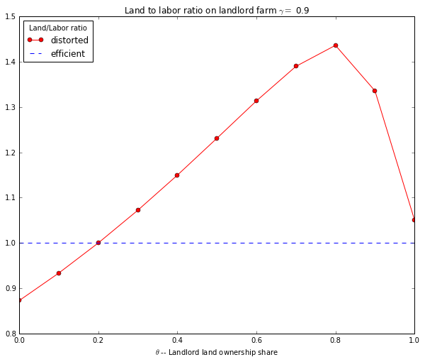
factor_plot(E,Xrc,Xr)

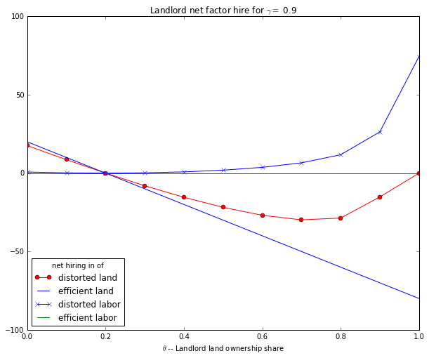
In the example above the ‘landlord’ farmer was in every way the same as the other farmers, the only difference being he had more land ownership (fraction \(\theta\) of the total). He had the same skill parameter as every other farmer. In an efficient equilibrium his operational farm size should therefore be the same size as every other farmer. The plot above shows how monopoly power (which rises with \(\theta\) allows the monopolist to distort the economy – he withholds land from the lease market to drive up the land rental rate and, since this deprives the ‘fringe’ of farmers of land, lowers the marginal product of labor on each smallholder farm, increasing the smallholder labor supply to the market which pushes down the labor wage. Hence we see how at higher levels of \(\theta\) the landlord expands the size of his estate and establish monopsony power wages.

A key force keeping the landlord from becoming too large is the fact that their are diseconomies of scale in production. THe landlord is expanding the scale of his operation (raising the land to labor ration on his farm in this example) earn more via distorted factor prices, but he balances off the increase in extraction from disorted wages against the cost of operating an inefficiently large farm (i.e. the cost of being too big).

Now let’s see the effect of making the landlord just a little bit more ‘skilled’ than the others. This lowers the cost of being big. But note that it also makes him bigger at lower theta and makes what I call the ‘size monopsony or ‘Feenstra’ effect matter more..

So let’s raise the landlord farmer’s productivity 10% relative to the rest of the farmers.

TLratio_plot(E,Xrc,Xr)

E.s[-1]=1.10

Let’s recalculate the new equilibria under the different scenarios.

(Xrc,Xr,wc,wr) = scene_print(E,10,detail=True)

Running 10 scenarios...

Assumed Parameters
==================
ALPHA  : 0.5 GAMMA  : 0.9 H      : 0.0 LAMBDA : 0.2
LBAR   : 100 N      : 5 TBAR   : 100 s      : [ 1.   1.   1.   1.   1.1]

Effcient:[ Trc, Lrc]      [rc,wc]       w/r    F( )    [r*Tr]  [w*Lr]
==============================================================================
        [ 39.34, 39.34]  [0.34,0.34]   1.00  | 29.97   13.49    13.49

Theta  [ Tr, Lr ]      [rM,wM]        w/r  | F()   [T_hire]  [T_sale] [L_hire]
==============================================================================
 0.00  [ 30.67, 35.14] [ 0.33, 0.35]  1.07 | 25.47    10.07     0.00    12.33
 0.10  [ 32.24, 34.54] [ 0.33, 0.35]  1.04 | 25.84    10.76     3.34    11.94
 0.20  [ 34.32, 34.32] [ 0.34, 0.34]  1.00 | 26.51    11.68     6.80    11.68
 0.30  [ 37.05, 34.56] [ 0.35, 0.33]  0.96 | 27.52    12.88    10.43    11.55
 0.40  [ 40.60, 35.31] [ 0.36, 0.33]  0.92 | 28.96    14.50    14.28    11.58
 0.50  [ 45.23, 36.74] [ 0.37, 0.32]  0.87 | 30.95    16.72    18.48    11.76
 0.60  [ 51.36, 39.10] [ 0.39, 0.31]  0.80 | 33.70    19.92    23.27    12.11
 0.70  [ 59.75, 42.98] [ 0.42, 0.29]  0.71 | 37.65    24.97    29.25    12.68
 0.80  [ 71.98, 50.11] [ 0.48, 0.27]  0.56 | 43.86    34.56    38.42    13.51
 0.90  [ 90.93, 68.06] [ 0.73, 0.21]  0.28 | 55.93    66.42    65.74    14.12
 0.99  [ 99.92, 95.08] [  4.1, 0.07]  0.02 | 67.82   411.11   407.35     6.74
==============================================================================

factor_plot(E,Xrc,Xr)

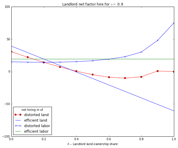
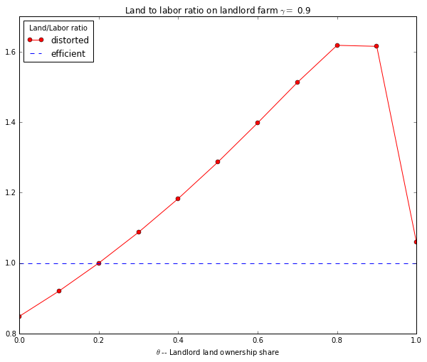
Given that he is more skilled than before the landlord’s efficient scale of production has increased. This lowers the cost of being big. Interestingly at low \(\theta\) this leads the landlord to hire less land and labor …

TLratio_plot(E,Xrc,Xr)