Farm Household Models

Most economics textbooks typically present the decisions of firms in separate chapters from the decisions of households. In this artificial but useful dichotomy the firm organizes production and hires factors of production while households own the factors of production (and ownership shares in firms). Households earn incomes from supplying these factors to firms and use that income to purchase products from the firms.

Many households in developing countries however may operate small farms, garden plots, stores or other types of businesses, and may also at the same time sell or hire labor in the labor market. In fact a large literature suggests that one defining characteristic of developing countries labor markets is the very large fraction of its labor force that are self-employed ‘own account’ workers and the many who run small businesses alongside wage labor jobs (Gollin, 2008).

For this reasin it will be useful to build models that allow households to both utilize labor and other factors as potential producers who may also choose to sell or hire these factors on factor markets. Here we offer stylized representations of the so called ‘farm household model’ or ‘agricultural household model’ (Singh, Squire, Strauss, 1986).

In these models the household acts both as a consumption unit, maximizing utility over consumption and ‘leisure’ choices and as a production unit, deciding how to allocate factors of production to the household farm or business.

A key question in this literature is whether the household’s production decisions (such as its choice of labor and other inputs and the scale of production) are separable or not from its preferences and endowments (e.g. consumer preferences, household demographic composition and ownership of land and other resources). For example, will a rural farm household with more working age adults run a larger farm compared to a neighboring household that is otherwise similar and has access to the same technology but has fewer working-age adults? If the households decisions are non-separable then the answer might be yes: the larger household uses of its larger labor force to run a larger farm.

When households are embedded in well functioning competitive markets however we tend to expect the household’s decisions to become separable:

• Household as a profit-maximizing firm: acting as a profit-maximizing firm the household first optimally chooses labor and other input allocations to extract maximum profit income from the farm.
• Household as a consumption unit: the household makes optimal choices over consumption and leisure subject to its income budget which includes income from selling its labor endowment and maximized profits from the household as a firm.

In the simple example above of two otherwise identical households the separable farm household model would predict that both households run farms of similar size and use wage labor markets to equalize land-labor ratios and hence marginal products of labor across farms. The larger household would be a net seller of labor on the market compared to the smaller household.

Without the separation property the common approach of many studies to separately estimate consumer demand from output supply functions is no longer valid.

Another way to state the separation hypothesis is that if they have access to markets the marginal production decisions of farms (and firms more generally) should not depend on their owners’ ownership of tradable factors (except in so far as it might raise their overal income) or their preferences in consumption. When markets are complete then production decisions will be separable, the price mechanism will equalize the marginal products of factors across uses, and the initial distribution of tradable factors should not matter for allocative efficiency (the first and second welfare theorems). Much of modern micro-development since at least the mid 1960s however is concerned with how transactions costs, asymmetric information, conflict and costly enforcement can lead to market frictions and imperfections that make production decisions non-separable, which then means that the initial distribution of property rights (over land and other tradable factors) may in fact well matter for determining the patterns of production organization and its efficiency in general equilibrium. A good example of such analysis is Eswaran and Kotwal (1986) paper on “Access to Capital and Agrarian production organization,” which explores how the combination of transaction costs in labor hiring and in access to capital can lead to a theory of endogenous class structure or occupational choice which can change dramatically depending on the initial distribution of property rights.

The Chayanovian Household

We’ll start with a non-separable model, inspired by the work of the Russian agronomist Alexander Chayanov whose early 20th century ideas and writings on “the peasant economy” became widely influential in anthropology, economics, and other fields. Chayanov played a role in the Soviet agrarian reforms but his focus on the importance of the household economy led him to be (presciently) skeptical of the appropriateness and efficiency of large-scale Soviet farms. He was arrested, sent to a labor camp and later executed.

The following model is not anywhere as rich as Chayanov’s description of the peasant household economy but instead a stripped down version close in spirit to Amartya Sen’s (1966) adaptation.

Farm household \(i\) has land and labor endowment \((\bar T_i, \bar L_i )\). We can assume that it can buy and sell the agricultural product at a market price \(p\) but in practice we will model the household as self-sufficient and cut off from the market for land and labor. The household (which we treat as a single decision-making unit for now) allocates labor maximizes utility over consumption and leisure

\[\max_{c_i,l_i} U(c_i,l_i)\]

Although we haven’t included it above, we think of the utility function \(U(c_i,l_i;A)\) as depending on ‘preference shifters’ \(A\) which might include such things as the household’s demographic composition or things that affect it’s preference for leisure over consumption).

The household maximizes this utility subject to the constraints that consumption \(c_i\) not exceed output and that the sum of hours in production \(L_i\) plus hours in leisure \(l_i\) not exceed the household’s labor endowment \(\bar L_i\)

\[c_i \leq F(\bar T_i, L_i)\]

\[L_i + l_i \leq \bar L_i\]

Substituting the constraints into the objective allows one to redefine the problem as one of choosing the right allocation of labor to production:

\[\max_{L_i} U(F(\bar T_i, L_i),\bar L_i - L_i)\]

From the first order necessary conditions we obtain

\[U_c \cdot F_L = U_l\]

which states that the farm household should allocated labor to farm production up to the point where the marginal utility benefit of additional consumption \(U_c \cdot F_L\) equals the opportunity cost of leisure.

Since the household sets the marginal product of labor (or shadow price of labor) equal to the marginal rate of substitution between leisure and consumption \(F_L = U_l/U_c\) and the latter is clearly affected by ‘preference shifters’ \(A\) and also by the household’s land endowment. The shadow price of labor will hence differ across households that are otherwise similar (say in their access to production technology and farming skill). For example households with a larger endowment of labor will run larger farms.

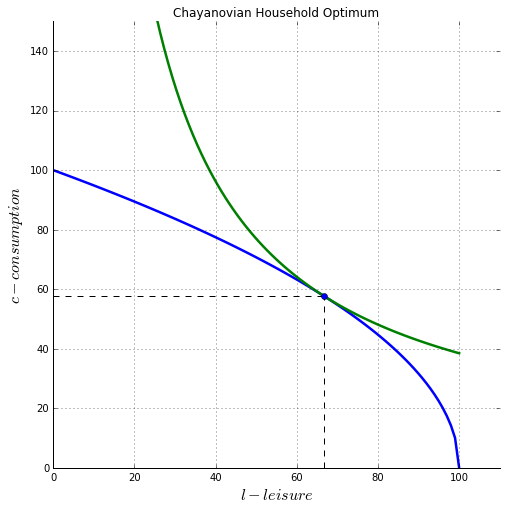
It will be useful to draw things in leisure-consumption space. Leisure is measured on the horizontal from left to right which then means that labor \(L\) allocated to production can be measured from right to left with an origin starting at the endowment point \(\bar L_i\)

To fix ideas with a concrete example assume farm household \(i\) has Cobb-Douglas preferences over consumption and leisure:

\[U(c,l) = c^\beta l^{1-\beta}\]

and its production technology is a simple constant returns to scale Cobb-Douglas production function of the form:

\[F(\bar T_i,L_i)=\bar T_i^\alpha L_i^{1-\alpha}\]

The marginal product of labor \(F_L\) which the literature frequently refers to as the shadow price of labor will be given by:

\[F_L (\bar T_i,L_i) = (1-\alpha) \left [ {\frac{\bar T_i}{L_i}} \right ]^\alpha\]

The first order necessary condition can therefore be solved for and for these Cobb-Douglas forms we get a rather simple and tidy solution to the optimal choice of leisure

\[l^* = \frac{a \cdot \bar L}{1+a}\]

where \(a=\frac{1-\beta}{\beta \cdot (1-\alpha)}\)

Graphical analysis

(Note: formulas and plots work for default parameters but not checked for other values.)

%matplotlib inline
import matplotlib.pyplot as plt
import numpy as np
from ipywidgets import interact

ALPHA = 0.5
BETA = 0.7
TBAR = 100
LBAR = 100

def F(T,L,alpha=ALPHA):
    return (T**alpha)*(L**(1-alpha))

def FL(T,L,alpha=ALPHA):
    """Shadow price of labor"""
    return (1-alpha)*F(T,L,alpha=ALPHA)/L

def FT(T,L,alpha=ALPHA):
    """Shadow price of labor"""
    return alpha*F(T,L,alpha=ALPHA)/T

def U(c, l, beta=BETA):
    return (c**beta)*(l**(1-beta))

def indif(l, ubar, beta=BETA):
    return ( ubar/(l**(1-beta)) )**(1/beta)

def leisure(Lbar,alpha=ALPHA, beta=BETA):
    a = (1-alpha)*beta/(1-beta)
    return Lbar/(1+a)

def HH(Tbar,Lbar,alpha=ALPHA, beta=BETA):
    """Household optimum leisure, consumption and utility"""
    a = (1-alpha)*beta/(1-beta)
    leisure = Lbar/(1+a)
    output = F(Tbar,Lbar-leisure, alpha)
    utility = U(output, leisure, beta)
    return leisure, output, utility

def chayanov(Tbar,Lbar,alpha=ALPHA, beta=BETA):
    leis = np.linspace(0.1,Lbar,num=100)
    q = F(Tbar,Lbar-leis,alpha)
    l_opt, Q, U = HH(Tbar, Lbar, alpha, beta)
    print("Leisure, Consumption, Utility =({:5.2f},{:5.2f},{:5.2f})"
          .format(l_opt, Q, U))
    print("shadow price labor:{:5.2f}".format(FL(Tbar,Lbar-l_opt,beta)))
    c = indif(leis,U,beta)
    fig, ax = plt.subplots(figsize=(8,8))
    ax.plot(leis, q, lw=2.5)
    ax.plot(leis, c, lw=2.5)
    ax.plot(l_opt,Q,'ob')
    ax.vlines(l_opt,0,Q, linestyles="dashed")
    ax.hlines(Q,0,l_opt, linestyles="dashed")
    ax.set_xlim(0, 110)
    ax.set_ylim(0, 150)
    ax.set_xlabel(r'$l - leisure$', fontsize=16)
    ax.set_ylabel('$c - consumption$', fontsize=16)
    ax.spines['right'].set_visible(False)
    ax.spines['top'].set_visible(False)
    ax.grid()
    ax.set_title("Chayanovian Household Optimum")
    plt.show()

chayanov(TBAR,LBAR,0.5,0.5)

Leisure, Consumption, Utility =(66.67,57.74,62.04)
shadow price labor: 0.87

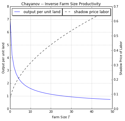
Inverse farm size productivity relationship

In this non-separable household with no market for land or labor, each household farms as much land as it owns. We find the well-known inverse farm size-productivity relationship: output per hectare is higher on smaller farms. Households with larger farms enjoy higher marginal products of labor – a higher shadow price of labor.

These two relationships can be seen below on this two-axis plot.

Tb = np.linspace(1,LBAR)
le, q, _ = HH(Tb,LBAR)
fig, ax1 = plt.subplots(figsize=(6,6))
ax1.plot(q/Tb,label='output per unit land')
ax1.set_title("Chayanov -- Inverse Farm Size Productivity")
ax1.set_xlabel('Farm Size '+r'$\bar T$')
ax1.set_ylabel('Output per unit land')
ax1.grid()
ax2 = ax1.twinx()
ax2.plot(FL(Tb,LBAR-le),'k--',label='shadow price labor')
ax2.set_ylabel('Shadow Price of Labor')
legend = ax1.legend(loc='upper left', shadow=True)
legend = ax2.legend(loc='upper right', shadow=True)
plt.show()

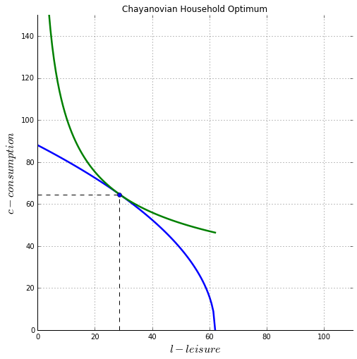
If you are running this notebook in interactive mode you can play with the sliders:

interact(chayanov,Tbar=(50,200,1),Lbar=(24,100,1),alpha=(0.1,0.9,0.1),beta=(0.1,0.9,0.1))

Leisure, Consumption, Utility =(28.62,64.60,50.60)
shadow price labor: 0.58

<function __main__.chayanov>

The Separable Farm Household

Consider now the case of the household that participates in markets. It can buy and sell the consumption good at market price \(p\) and buy or sell labor at market wage \(w\). Hired labor and own household labor are assumed to be perfect substitutes.

To keep the analysis a little bit simpler and fit everything on a single graph we’ll assume that the market for land leases remains closed. However it is easy to show that for a linear homogenous production function this will not matter for allocative efficiency – it will be enough to have a working competitive labor market for the marginal product of land and labor to equalize across farms.

When the farm household is a price-taker on markets like this, farm production decisions become ‘separable’ from farm consumption decisions. The farm household can make its optimal decisions as a profit-maximizing farm and then separately choose between consumption and leisure subject to an income constraint.

So the household’s problem can be boiled down to:

\[ \begin{align}\begin{aligned}\max_{c,l} U(c,l)\\s.t.\end{aligned}\end{align} \]

\[p \cdot c \leq pF(\bar T_i,L^*) + w \cdot (\bar L_i - l)\]

This last constraint states that what the household spends on consumption cannot exceed the value of farm sales at a profit maximizing optimum plus wage income from labor sold to the market. This last constraint can also be rewritten as:

\[p \cdot c + w \cdot l \leq \Pi (T_i,w,p) + w \cdot \bar L_i\]

where \(\Pi (T_i,w,p) = p \cdot F(T_i,L^*_i) - w \cdot L^*_i\) is the maximized value of farm profits and \(L^*_i\) is the optimal quantity of labor that achieves that maximum.

In other words the farm household can be thought of as maximizing profits by choosing an optimal labor input into the farm \(L^*_i\) which will be satisfied with own and/or hired labor. The household then maximizes utility from consumption and leisure subject to the constraint that it not spend more on consumption and leisure as its income which is made up of farm profits (a return to land) and the market value of it’s labor endowment.

In this last description the household is thought of as buying leisure at its market wage opportunity cost.

The efficient competitive farm

As a production enterprise the farm acts to maximize farm profits $pF(

\bar

T_i,L_i) - w

\cdot

L_i $. The first-order necessary condition for an interior optimum is:

\[p \cdot F_L (\bar T_i,L) = w\]

The separation property is immediately apparent from this first order condition, as this equation alone is enough to determine the farm’s optimum labor demand which depends only on the production technology and the market wage, and not at all on household preferences. While the quantity of labor demanded here does depend on the households’ ownership of land, with a functioning labor market the number of workers per unit land will be the same across all farms and hence also independent of household land endowment.

For the Cobb-Douglas production function, optimal labor demand can then be solved to be:

\[L_i^* = \bar T_i \cdot \left [ {\frac{p(1-\alpha)}{w}} \right ]^\frac{1}{\alpha}\]

Substituting this value into the profit function we can find an expression for farm profits \(\Pi (T_i,w,p)\) as a function of the market product price and wage and the farm’s land holding. If we had allowed for hiring on both land and labor markets we would have found zero profits with this linear homogenous technology so in this context where there is no working land market, profits are just like a competitively determined rent to non-traded land (equal in value to what the same household would have earned on its land endowment had the land market been open).

Note how the optimal allocation of labor to the farm is independent of the size of the household \(\bar L_i\) and household preferences. If we had allowed for a competitive land market the labor allocation would also have been independent of the household’s

Household demand for consumption and leisure is very simple given this Cobb-Douglas utility:

\[c^*(w) = \beta \cdot I\]

\[l^*(w) = (1-\beta) \cdot \frac{I}{w}\]

where household income \(I\) is given by the sum of farm profits and the market value of the factor endowment:

\[I = \Pi(w,\bar T) + w \cdot \bar L\]

In what follows we shall normalize the product price \(p\) to unity. This is without loss of generality as all that matters for real allocations is the relative price of labor (or leisure) relative to output, or the real wage \(\frac{w}{p}\). So in all the expressions that follow when we see \(w\) it should be thought of as \(\frac{w}{p}\)

def farm_optimum(Tbar, w, alpha=ALPHA, beta=BETA):
    """returns optimal labor demand and profits"""
    LD = Tbar * ((1-alpha)/w)**(1/alpha)
    profit = F(Tbar, LD) - w*LD
    return LD, profit

def HH_optimum(Tbar, Lbar, w, alpha=ALPHA, beta=BETA):
    """returns optimal consumption, leisure and utility.
       Simple Cobb-Douglas choices from calculated income """
    _, profits = farm_optimum(Tbar, w, alpha)
    income = profits + w*Lbar
    consumption = beta * income
    leisure = (1-beta) * income/w
    utility = U(consumption, leisure, beta)
    return consumption, leisure, utility

Let’s assume the market real wage starts at unity:

W = 1

def plot_production(Tbar,Lbar,w):
    lei = np.linspace(1, Lbar)
    q = F(Tbar, Lbar-lei)
    ax.plot(lei, q, lw=2.5)
    ax.spines['right'].set_visible(False)
    ax.spines['top'].set_visible(False)

def plot_farmconsumption(Tbar, Lbar, w, alpha=ALPHA, beta=BETA):
    lei = np.linspace(1, Lbar)
    LD, profits = farm_optimum(Tbar, w)
    q_opt = F(Tbar,LD)
    yline = profits + w*Lbar - w*lei
    c_opt, l_opt, u_opt = HH_optimum(Tbar, Lbar, w)

    ax.plot(Lbar-LD,q_opt,'ob')
    ax.plot(lei, yline)
    ax.plot(lei, indif(lei,u_opt, beta),'k')
    ax.plot(l_opt, c_opt,'ob')
    ax.vlines(l_opt,0,c_opt, linestyles="dashed")
    ax.hlines(c_opt,0,l_opt, linestyles="dashed")
    ax.vlines(Lbar - LD,0,q_opt, linestyles="dashed")
    ax.hlines(profits,0,Lbar, linestyles="dashed")
    ax.vlines(Lbar,0,F(Tbar,Lbar))
    ax.hlines(q_opt,0,Lbar, linestyles="dashed")
    ax.text(Lbar+1,profits,r'$\Pi ^*$',fontsize=16)
    ax.text(Lbar+1,q_opt,r'$F(\bar T, L^{*})$',fontsize=16)
    ax.text(-6,c_opt,r'$c^*$',fontsize=16)

    ax.annotate('',(Lbar-LD,2),(Lbar,2),arrowprops={'arrowstyle':'->'})
    ax.text((2*Lbar-LD)/2,3,r'$L^{*}$',fontsize=16)

    ax.text(l_opt/2,8,'$l^*$',fontsize=16)
    ax.annotate('',(0,7),(l_opt,7),arrowprops={'arrowstyle':'<-'})

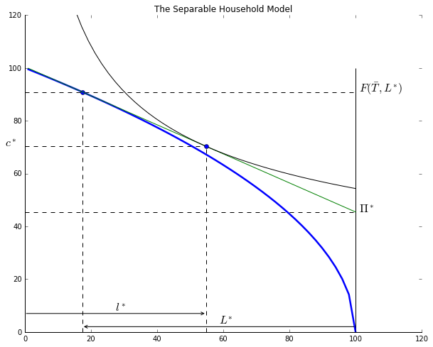
Here is an example of a household that works and their own farm and sells labor to the market:

fig, ax = plt.subplots(figsize=(10,8))
plot_production(TBAR,LBAR,W)
plot_farmconsumption(TBAR, LBAR, W)
ax.set_title("The Separable Household Model")
ax.set_xlim(0,LBAR+20)
ax.set_ylim(0,F(TBAR,LBAR)+20)
plt.show()

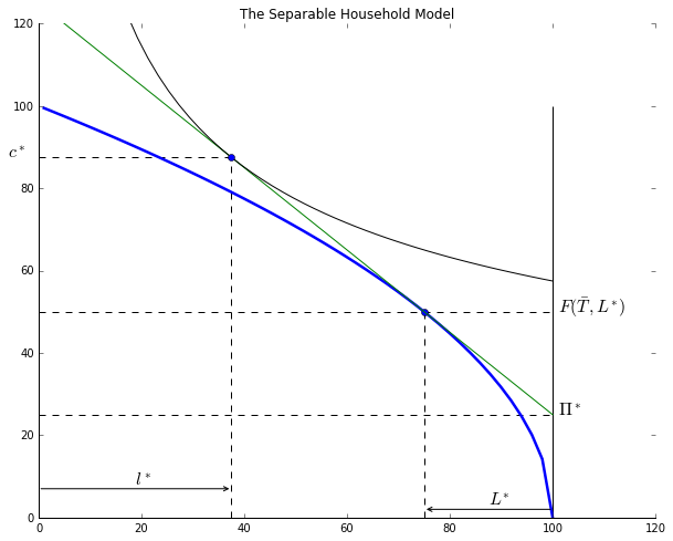
Here is the same household when facing a much lower wage (55% of the wage above). They will want to expand output on their own farm and cut back on labor sold to the market (expand leisure). This household will on net hire workers to operate their farm.

fig, ax = plt.subplots(figsize=(10,8))
plot_production(TBAR,LBAR, W*0.55)
plot_farmconsumption(TBAR, LBAR, W*0.55)
ax.set_title("The Separable Household Model")
ax.set_xlim(0,LBAR+20)
ax.set_ylim(0,F(TBAR,LBAR)+20)
plt.show()

No Inverse farm size productivity relationship

Since every farm takes the market wage as given the marginal product of labor will be equalized across farms. The shadow price of labor will equal the market wage on all farms, regardless of their land size. The land labor ratio and hence also the marginal product of land will also equalize across farms so output per unit land will also remain constant.

The next section describes some empirical tests of the separation hypothesis as well as models with ‘selective-separability’ where missing markets and/or transactions costs end up determining that, depending on their initial ownership of assets, some households may face different factor shadow prices depending on whether they are buyers or sellers or non-participants on factor markets.

This last example should drive home the point that when the farm household’s optimization problem is separable the farm’s optimal choice of inputs will be independent of both household characteristics and it’s endownment of tradable factors such as land and labor.

In this last example when we shut down the labor market and introduce a transaction wedge on the market for land we create a non-separable region of autarkic or non-transacting households (shaded above). A framework such as this would generate data that displays the classic inverse farm-size productivity relationship. Farms that lease in land are smaller and have higher output per hectare than larger farms that lease land out and within the autarky zone farm size is increasing in the size of the land endowment and the shadow price (and hence output per unit land) falling.