Testing for Separation in Household models

There are a few related approaches to testing for separation. The early studies were ‘global’ tests that aimed at accepting or rejecting the null hypothesis of a separable household model for the entire sample of households. Some later studies argue that a more typical situation is one where only ‘local’ subsets of households may be constrained and therefore caught in a ‘non-separable’ regime and that any econometric estimation strategy should be sensitive to this fact.

Global separation tests:

One approach attempts to test the implication of the separation hypothesis that labor demand should be independent of household preference shifters \(A\) (i.e. demographic characteristics of the household. Basically this approach regresses labor demand on prices, fixed non-traded inputs, and a measure of \(A\). The null hypothesis is that the model is separable and the coefficient on A is zero. Therefore an insignificant estimated coefficient is interpreted as a failure to reject the null hypothesis of separation. There are econometric issues such as simultaneity bias to worry about of couse. This is the approach of papers such as Lopez (1984), Benjamin (1992) and many others.

Another approach builds from the observation that under separation the shadow price of labor or the marginal product of labor on the farm – call it \(w^*\) – should equal the market wage \(w\). Since the shadow wage is not directly observed it must be calculated off an estimated production function. If estimates of \(w*\) have been estimated across farms the separation test boils down to a test of whether \(\beta_0 = 0\) and \(\beta_1 =1\) in the regression \(w^* = \beta_0 +\beta_1 w\). Issues of endogeneity and other econometic concerns must be addressed. This is the approach of Jacoby (1993), Skoufias (1994) and others.

Kien Le (2010) proposes a semi-parametric method that combines elements of both of the above approaches but uses less data. his apprach boils down to regressing the log of the measured value of output per worker on each farm against the market wage and a few controls.

Selective-separability

A small but important literature attempts to model farm household behavior on markets with transactions costs. The basic idea is that transactions costs such as the cost of getting to work can establish a wedge between the cost of hiring and selling labor. Suppose for example that farms that hire have to pay workers a wage of \(w\) per hour but workers take home only \(w(1-\tau)\) of the wage due to transaction costs. If a would-be worker has the option of operating their own farm it should be clear that they would work sell their labor to the market as long as the shadow price (marginal product) of labor on their own farm falls below \(w(1-\tau)\), they will neither hire nor sell labor to the market if the shadow price of labor is above \(w(1-\tau)\) but below \(w\) and they will hire labor if the shadow price is above \(w\). In a simple model where other factors of production (say land or farming skill) are missing then households may be placed into each of these three regimes (hiring out, self-sufficient, hiring in) depending on the initial distribution of these non-traded assets across households. The extent of allocative inefficiency (misallocation compared to the same economy without transaction costs) will depend on both the size of the transaction costs and the initial distribution of non-traded assets. In the simple model I’ve just traced out households that operate farms and also hire out labor will in general be producing using more labor-intensive methods compare to households that hire-in labor since the latter face a higher wage.

de Janvry et al (1991) highlight some of the many ‘puzzles’ and behaviors that can be explained by adding transaction costs to an otherwise neoclassical model. Sadoulet et al (1996) appear to be one of the earliest, if not the earliest paper to use the term ‘selective separability’ to refer to this fact that households may be selectively in one regime or another, depending on their asset holdings.

Carter and Yao (2002): Local versus Global Separability

Carter and Yao’s (2002) paper “Local versus Global Separability in Agricultural Household Models: The factor price equalizaiton effect fof land transfer rights,” offers an example of local versus global separability tests. They consider a model where transaction costs establish a wedge between the rental rate tenants must pay to hire-in land and the rental rate that landlords receive for hiring-out land. In a relatively simple model where the labor market is closed (which they argue fits their Chinese panel dataset from 1988 and 1993) this situation will generate a three regime equilibrium: (1) households with an endowment ratio of land relative to labor below some threshold will be tenants and hire-in land but these households are price-takers and the regime is separable in that all households in this group employ a common high labor intensity and low shadow wage. (2) households with an endowment ratio above a different higher threshold will rent-out land and are also in a separable regime but with a lower labor-land intensity and higher shadow wage. Finally households in the non-separable autarky regime (3) are those with endowment ratios between the two thresholds; these households do not hire in or hire out land but instead employ the land they have which means that for households in this group the shadow wage rises with the endowment ratio.

As the authors point out, referring to earlier ‘global’ tests:

…neither separability, nor non-separability exist globally across the full endowment continuum …the reduced form global separability tests found in the econometrics literature (which do not distinguish between rental regimes) would be mis-specified and subject to a degree of bias that depends on the distribution of households across the three regimes.

They employ a switching regression approach where the model of labor intensity to be estimated depends on the discrete rental regime a household is classified into. The authors employ a simulated MLE method to estimate the system with panel data. They contrast their estimates with what would be found on the same dataset with one of the global tests of separability, arguing that the results from a global test are biased and misleading.

Carter and Yao’s (2002) paper “Local versus Global Separability in Agricultural Household Models: The Factor Price Equalization Effect of Land Transfer Rights”

were analyzing households in rural China in the late 80s and 90s, a period of transition where land markets were being slowly liberalized. The authors describe the situation as one where it was reasonable to assume no market for wage labor and a limited market for land. They model this last idea as a wedge between the rental rate that is received by households that lease out land \(r^O = r(1-c^O(M))\) and the amount that households had to pay to rent land in \(r^I= r(1+c^I(M))\), where \(r^O \leq r \leq r^I\).

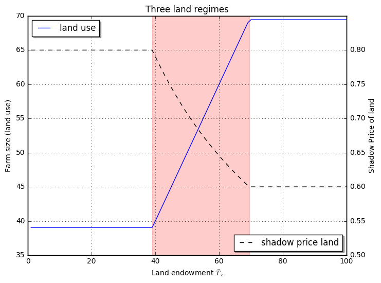
To see this clearly, suppose households (HH) are otherwise identical to each other in all respects – including the size of their labor force, call it \(\bar L_e\) – and only differ in terms of their endowment of land \(T_i\). Households can then be classified as belonging to one of three behavioral regimes, depending the relative size of their land endowment.

, two where household behavior can be characterized as separable, and one w.

1. HH that rent-in land, :math:`T_i in (0,T^I]`: Households with a low endowment of land will lease in land at the high rent-in market rate \(r^I\) to operate a farm of size \(T^I\).
2. HH in autarky, :math:`T_i in (T_I,T^O]`: Households with a land endowment withing these two thresholds will operate their own land at shadow rate \(r^0<r^*< r^I\).
3. HH that rent-out land, :math:`T_i in [T_O,bar T]`: Households with a high endowment of land will lease out land at the low rent-out market rate \(r^O\) and operate a farm of size \(T^O\).

Leaving aside the issue of how the equilibrium rental rate is determined (discussed in other sections) suppose \(r^I\) and \(r^O\) are given. Then Households in the first regime operate farms of size maximize farm profits

\[p \cdot F_T (T^I,\bar L_e) = r^I\]

Households in the third regime operate farms of size maximize farm profits

\[p \cdot F_T (T^O,\bar L_e) = r^O\]

And farms with a land endowment of \(T_i \in (T_I,T^O]\) will operate a farm of size \(T_i\) and the shadow rental rate of land on their farm will be

\[r^*(T_i) = p \cdot F_T (T_i,\bar L_e)\]

Below is a plot for our simple Cobb-Douglass example and reasonable parameter values.

%matplotlib inline
import matplotlib.pyplot as plt
import numpy as np

ALPHA = 0.5
BETA = 0.7
TBAR = 100
LBAR = 100

def F(T,L,alpha=ALPHA):
    return (T**alpha)*(L**(1-alpha))

def FT(T,L,alpha=ALPHA):
    """Shadow price of labor"""
    return alpha*F(T,L,alpha=ALPHA)/T

def yao_carter(Ti, rO, rI, alpha=ALPHA):
    """returns optimal land use and shadow rental price of land"""
    r = FT(Ti, LBAR, alpha)
    Tout = LBAR * (alpha/rO)**(1/(1-alpha))
    Tin = LBAR * (alpha/rI)**(1/(1-alpha))
    TD = (r < rO)*Tout + (r > rI)* Tin  + ((r>=rO) & (r<=rI))*Ti
    rs = (r < rO)*rO + (r > rI)* rI  + ((r>=rO) & (r<=rI)) * r
    fig, ax1 = plt.subplots(figsize=(8,6))
    ax1.plot(Ti,TD,label='land use')
    ax1.set_title("Three land regimes")
    ax1.set_xlabel('Land endowment '+r'$\bar T_e$')
    ax1.set_ylabel('Farm size (land use)')
    ax1.grid()
    ax2 = ax1.twinx()
    ax2.plot(Ti, rs,'k--',label='shadow price land')
    ax2.set_ylabel('Shadow Price of land')
    ax2.set_ylim(0.5,0.85)
    ax1.axvspan(Tin, Tout, alpha=0.2, color='red')
    legend = ax1.legend(loc='upper left', shadow=True)
    legend = ax2.legend(loc='lower right', shadow=True)
    plt.show()

Ti = np.linspace(1,TBAR,num=100)
RI = 0.8
RO = 0.6
yao_carter(Ti, RO, RI, alpha=ALPHA)