Coase, Property rights and the ‘Coase Theorem’¶

Coase, R. H. 1960. “The Problem of Social Cost.” The Journal of Law and Economics 3:1–44.

Coase, Ronald H. 1937. “The Nature of the Firm.” Economica 4 (16):386–405.

Note: Most of the code to generate visuals and results below is in a code section at the end of this notebook. To run interactive widgets or modify content, navigate to the code section for instructions.

Slideshow mode: this notebook can be viewed as a slideshow by pressing Alt-R if run on a server.

Coase (1960)¶

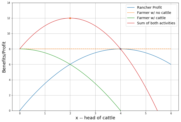
A rancher and wheat farmer.¶

Both are utilizing adjacent plots of land. There is no fence separating the lands.

The Wheat Farmer

The wheat farm choose a production method the delivers a maximum profit of $\Pi_W =8$. - to keep this simple suppose this is the farmer’s only production choice.

The Rancher

Chooses herd size $x$ to maximize profits:

\[\Pi_C(x) = P \cdot F(x) - c \cdot x\]

where $P$ is cattle price and $c$ is the cost of feeding each animal.

To simplify we allow decimal levels (but conclusions would hardly change if restrictedto integers).

First-order necessary condition for herd size $x^*$ to max profits:

\[P \cdot F'(x^*) = c\]

**Example:* $P_c=4$, $F(x) = \sqrt{x}$ and $c=1$

The FOC are $\frac{4}{2\sqrt x*} = 1$

And the rancher’s privately optimal herd size:

\[x^* = 4\]

The external cost

No effective barrier exists between the fields so cattle sometimes strays into the wheat farmer’s fields, trampling crops and reducing wheat farmer’s profits.

Specifically, if rancher keeps a herd size $x$ net profits in wheat are reduced to :

\[\Pi_W(x) = \Pi_W - d \cdot x^2\]

The external cost

Suppose $d=\frac{1}{2}$

At rancher’s private optimum herd size of $x*=4$ the farmer’s profit is reduced from 8 to zero:

\[\begin{split}\begin{align} \Pi_W(x) &= \Pi_W - d \cdot x^2 \\ & = 8 - \frac{1}{2} \cdot 4^2 = 0 \end{align}\end{split}\]

In [11]:

Pc = 4
Pw = 8
c = 1/2
d = 1/2

CE, TE = copt(),topt()
CE, TE

Out[11]:

(4.0, 2.0)

If the rancher chose his private optimum he’d earn $8 but drive the farmer’s earnings to zero.

In [12]:

coaseplot1()

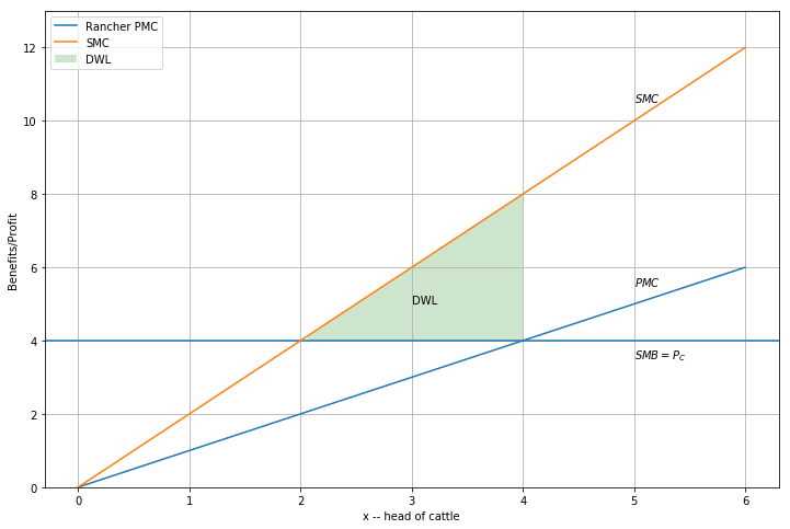
Private and social marginal benefits and costs can be plotted to see deadweight loss (DWL) differently:

In [13]:

coaseplot2()

The assignment of property rights (liability)¶

Scenario 1: Farmer has right to enjoin cattle herding (prohibit via an injunction).

Rancher now earns $0. Farmer $8.

This is not efficient either.

If rancher herded just 2 would earn $6. Could offer $2 compensation to the wheat farmer and capture $6-2 =$4.

…or they could bargain to divide the gains to trade of $4 in other ways.

Scenario 2: Rancher has right to graze with impunity.

Farmer earns $0 if rancher herds private optimal of 4 cattle. Farmer could offer to pay $2 to have rancher reduce herd to 2 which would leave rancher as well off and take the farmer from $0 to $4 (= 6-2).

…or they could bargain to divide the gains to trade of $4 in other ways.

With zero transactions costs¶

The initial assignment of property rights does not matter: The parties bargain to an efficient outcome either way.
However, like any scarce resource, legal rights are valuable, so **the initial allocation will affect the distribution of benefits and incomes between parties*
The emergence of property rights: Even if there is no initial assignment of property rights, with zero transactions costs it should be in the interests of the parties to negotiate to an efficient outcome.

With positive transactions costs¶

The initial distribution of property rights typically will matter.
It’s not so clear from this example but suppose that we had a situation with one wheat farmer and many ranchers. It might be difficult to get the ranchers

Coase and the development of a land market¶

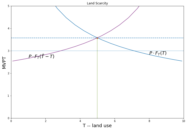
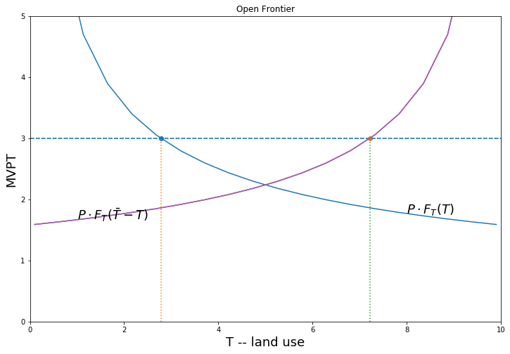
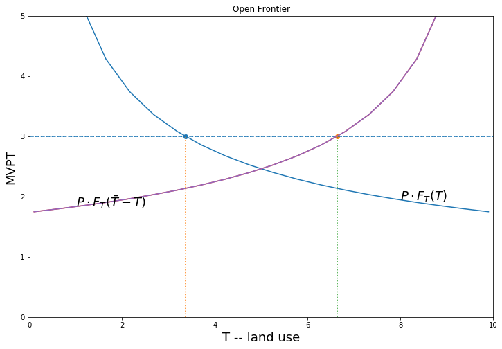
Suppose there is an open field. In the absence of a land market whoever gets to the land first (possibly the more powerful in the the village) will prepare/clear land until the marginal value product of the last unit of land is equal to the clearing cost. We contrast two situations:

Open frontier: where land is still abundant
Land Scarcity.

There will be a misallocation in (2) shown by DWL in the diagram… but also an incentive for the parties to bargain to a more efficient outcome. A well functionining land market would also deliver that outcome.

Abundant land environment

$\bar T$ units of land and $N$=2 households.

Land clearing cost $c$. Frontier land not yet exhausted.

Maximize profits at $P \cdot F_T(T) = c$

In [26]:

landmarket(P=5, cl = 3, title = 'Open Frontier')

In [27]:

landmarket(P=8, cl = 3, title = 'Land Scarcity')

The ‘Coase Theorem’¶

Costless bargaining between the parties will lead to an efficient outcome regardless of which party is awarded the rights?

Coase Theorem: True, False or Tautology?¶

Tautology?: “if there are no costs to fixing things, then things will be fixed.”

Like the First Welfare Theorem (complete competitive markets will lead to efficient allocations, regardless of initial allocation of property rights). The Coase Theorem makes legal entitlements tradable

Further notes on Coase (incomplete)¶

Coase can be seen as generalizing the neo-classical propositions about the exchange of goods (i.e. 1st Welfare Theorem) to the exchange of legal entitlements (Cooter, 1990). “The initial allocation of legal enttilements dos not matter foram an efficiency perspetive so long as they can be freely exchanged…’

Suggests insuring efficiency of law is matter or removing impediments to free exchange of legal entitlements…… define entitlements clearly and enforce private contracts for their exchagne…

But conditions needed for efficient resource allocation…

Nice discussion here:

Tautology: “Costless bargaining is efficient tautologically; if I assume people can agree on socially efficient bargains, then of course they will” “The fact that side payments can be agreed upon is true even when there are no property rights at all.” ” In the absence of property rights, a bargain establishes a contract between parties with novel rights that needn’t exist ex-ante.”

“The interesting case is when transaction costs make bargaining difficult. What you should take from Coase is that social efficiency can be enhanced by institutions (including the firm!) which allow socially efficient bargains to be reached by removing restrictive transaction costs, and particularly that the assignment of property rights to different parties can either help or hinder those institutions.”

Transactions cost: time and effort to carry out a transaction.. any resources needed to negotiate and enforce contracts…

Coase: initial allocation of legal entitlements does not matter from an efficiency perspective so long as transaction costs of exchange are nil…

Like frictionless plane in Phyisics… a logical construction rather than something encountered in real life..

Legal procedure to ‘lubricate’ exchange rather than allocate legal entitlement efficiently in the first place…

As with ordinary goods the gains from legal

The Political Coase Theorem¶

Acemoglu, Daron. 2003. “Why Not a Political Coase Theorem? Social Conflict, Commitment, and Politics.” Journal of Comparative Economics 31 (4):620–652.

Incomplete contracts¶

Hard to think of all contingencies
Hard to negotiate all contingencies
Hard to write contracts to cover all contingencies

Incomplete contracts - silent about parties’ obligations in some states or state these only coarsely or ambiguosly

Incomplete contracts will be revised and renegotiated as future unfolds…This implies
- ex-post costs (my fail to reach agreement..).
- ex-ante costs

Relationship-specific investments.. Party may be reluctant to invest because fears expropriation by the other party at recontracting stage.. - hold up: after tenant has made investment it is sunk, landlord may hike rent to match higher value of property (entirely due to tenant investment)… Expecting this tenant may not invest..

“Ownership – or power – is distributed among the parties to maximise their investment incentives. Hart and Moore show that complementarities between the assets and the parties have important implications. If the assets are so complementary that they are productive only when used together, they should have a single owner. Separating such complementary assets does not give power to anybody, while when the assets have a single owner, the owner has power and improved incentives.”

## Code Section Note: To re-create or modify any content go to the

‘Cell’ menu above run all code cells below by choosing ‘Run All Below’. Then ‘Run all Above’ to recreate all output above (or go to the top and step through each code cell manually).

In [1]:

import numpy as np
import matplotlib.pyplot as plt
from scipy.optimize import fsolve
%matplotlib inline

Default parameter values:

In [2]:

Pc = 4
Pw = 8
c = 1/2
d = 1/2

In [3]:

def F(x,P=Pc,c=c):
    '''Cattle Profit'''
    return P*x - c*x**2

def AG(x, P=Pw):
    '''Wheat farm profit before crop damage'''
    return P*(x**0)   # to return an array of len(x)

def AGD(x,P=Pw,d=d):
    return AG(x,P) - d*x**2

In [4]:

def copt(P=Pc,c=c):
    '''rancher private optimum'''
    return P/(2*c)

def topt(P=Pc,c=c, d=d):
    '''Social effient optimum'''
    return P/(2*(c+d))

In [5]:

CE, TE = copt(),topt()
CE, TE

Out[5]:

(4.0, 2.0)

In [6]:

xx = np.linspace(0,6,100)

In [7]:

def coaseplot1():
    fig = plt.subplots(figsize=(12,8))
    plt.plot(xx, F(xx), label = 'Rancher Profit' )
    plt.plot(xx, AG(xx), '--', label = 'Farmer w/ no cattle' )
    plt.plot(xx, AGD(xx), label = 'Farmer w/ cattle')
    plt.plot(xx, F(xx) + AGD(xx),label='Sum of both activities')
    plt.scatter(copt(),F(copt()))
    plt.scatter(topt(),F(topt()) + AGD(topt()))
    plt.grid()
    plt.ylim(0,14)
    plt.xlabel('x -- head of cattle', fontsize=18)
    plt.ylabel('Benefits/Profit', fontsize=18)
    plt.legend(fontsize=14);

In [8]:

coaseplot1()

Let’s plot a standard ‘external cost’ diagram

In [9]:

def MC(x,c=1/2):
    '''Cattle MC'''
    return 2*c*x

def excost(x,d=1/2):
    return 2*d*x

In [10]:

def coaseplot2(Pw=Pw, Pc=Pc):
    fig = plt.subplots(figsize=(12,8))
    plt.axhline(Pc);
    plt.plot(xx, MC(xx), label = 'Rancher PMC' )
    plt.plot(xx, MC(xx)+excost(xx), label = 'SMC')
    plt.fill_between(xx, MC(xx)+excost(xx),Pc*xx**0, where=((MC(xx)<=Pc*xx**0) & (xx>2)),
                     facecolor='green', alpha=0.2, label='DWL')

    plt.text(3,5,'DWL' )
    plt.text(5,3.5,r'$SMB = P_C$')
    plt.text(5,5.5, r'$PMC$')
    plt.text(5,10.5, r'$SMC$')
    #plt.scatter(topt(),G(topt()) + AGD(topt()))
    plt.grid()
    plt.ylim(0,13)
    plt.xlabel('x -- head of cattle')
    plt.ylabel('Benefits/Profit')
    plt.legend();

In [14]:

A=1

In [15]:

def F(T, A=A):
    return A*np.sqrt(T)

In [16]:

def MVPT(P,T,A=A):
    return A*P/T**(1/2)

def LD(P,r,A=A):
    return (P*A/r)**2

In [17]:

A=1
Tbar  = 10  # Total land endowment
P = 5.5     # Price of output
cl = 3      # cost of clearing land

Land demand for each farmer is given by $P\cdot F_T(T_i) = r$. So for this production $P \frac{1}{\sqrt T_i} = r$ or $P \frac{1}{\sqrt T_i} = cl$ so we can write

\[T^*_i(r) = (P/r)^2\]

If there is an open frontier the sum or demands falls short of total land supply and the marginal cost of land is the cost of clearing $r=c_l$. ‘Land scarcity’ results when there is an equilibrium price of land and$r>c_l$ where $r$ is found from

\[\sum T^*_i(r) = \bar T\]

In [18]:

def req(P,cl, Tb=Tbar, N=2, A=A):
    '''equilibrium rental rate'''
    def landemand(r):
        return N*(A*P/r)**2 - Tb
    return fsolve(landemand, 1)[0]

In [19]:

P, cl, req(P,cl)

Out[19]:

(5.5, 3, 2.4596747752497685)

In [20]:

LD(P, req(P,cl))*2, Tbar

Out[20]:

(10.000000000000002, 10)

In [21]:

def mopt(P,cl,A=A):
    '''Optimum land use for each i at the P*MPT = max(cl,r)'''
    r = req(P,cl)
    ru = max(cl, r)
    return (A*P/ru)**2

Farmer A will demand

In [22]:

mopt(P,cl), MVPT(P, mopt(P,cl) )

Out[22]:

(3.3611111111111107, 3.0)

In [23]:

#plt.style.use('bmh')

def landmarket(P, cl, title, A=A):
    t = np.linspace(0.1,Tbar-0.1, 2*Tbar)
    fig = plt.subplots(figsize=(12,8))
    x0 = mopt(P,cl,A=A)
    plt.ylim(0,5)
    #plt.axhline(cl,linestyle=':')
    plt.axhline(max(cl,req(P,cl,A=A)),linestyle='--')
    plt.axhline(cl,linestyle=':')
    plt.plot(t,MVPT(P,t))
    plt.text(8, MVPT(P,8),r'$P \cdot F_T(T)$', fontsize=18)
    plt.text(1, MVPT(P,Tbar-1),r'$P \cdot F_T(\bar T - T)$', fontsize=18)
    plt.xlabel('T -- land use', fontsize=18)
    plt.ylabel('MVPT', fontsize=18)

    plt.scatter(x0, MVPT(P,x0))
    plt.scatter(Tbar-mopt(P,cl),MVPT(P,x0))
    plt.plot([x0,x0],[0,MVPT(P,x0)],':')
    plt.plot([Tbar-x0,Tbar-x0],[0,MVPT(P,x0)],':')
    plt.plot(t,MVPT(P,Tbar - t))
    plt.plot(t,MVPT(P,Tbar-t))
    plt.title(title)
    plt.xlim(0,Tbar);

In [24]:

landmarket(P=5.5, cl = 3, title = 'Open Frontier')

In [25]:

landmarket(P=8, cl = 3, title = 'Land Scarcity')