The Specific Factors or Ricardo-Viner Model

Background

The SF model is a workhorse model in trade, growth, political economy and development. We will see variants of the model used to describe rural to urban migration, the Lewis model and other dual sector models of sectoral misallocation, models such as the Harris-Todaro model that explain migration and the urban informal sector. The specific factors model predicts that, in the absence of political redistribution mechanisms, specific factors in declining sectors will organize strong opposition to policies that might otherwise raise growth. The initial distribution of factor endowments may therefore make a big difference in terms of what types of political coalitions mobilize for and against different policies. This is the basic driving force in Moav-Galor’s (2006) growth model on why some regions made public investments in human capital which sped the transition from agriculture to manufacturing and enhanced growth, whereas similar policies were delayed in other regions where political/economic resistance was stronger, for instance where landlords had stronger voice in political decisions.

These are just a few of the applications. The model is relatively easy to analyze – it can be described compactly in terms of diagrams and yet is very rich in predictions.

The Specific Factors (SF) or Ricardo-Viner model is a close relative of the Hecksher-Ohlin-Samuelson (HOS) neoclassical trade model. The 2x2 HOS model assumes production in each of two sectors takes place by firms using constant returns to scale technologies with capital and labor as inputs and that both capital and labor are mobile across sectors. In the SF model only labor is inter-sectorally mobile and the fixed amounts of capital become ‘specific’ to the sector they are trapped within.

In effect the SF model therefore consists of three factors of production: mobile labor and two types of capital, one specific to each sector. Let’s label the two sectors are Agriculture and Manufacturing. In agriculture competitive firms bid to hire land and labor. In manufacturing competitive firms bid to hire capital and labor. Each factor of production will be competitively priced in equilibrium but only labor is priced on a national labor market.

The SF model is often described as a short-run version of the HOS model. For example suppose we start with a HOS model equilibrium where labor wage and rental rate of capital have equalized across sectors (which also implies marginal products are equalized across sectors – no productivity differences across sectors). Now suppose that the relative price of manufacturing products suddenly rises (due to a change of world price, or government trade protection or other policies that favor manufacturing). The higher relative product price should lead firms in the booming manufacturing sector to demand both more capital and labor. Correspondingly, demand for land and labor decline in the agricultural sector. In the short run however only labor can be move from agriculture to manufacturing. Agricultural workers can become factory workers but agricultural capital (say ‘land’ or ‘tractors’) cannot be easily converted to manufacturing capital (say ‘weaving machines’). So labor moves from manufacturing to the agriculture, lowering the capital labor ratio in manufacturing and raising the land to labor ratio in agriculture. The model thus predicts a surge in the real return to capital in the expanding sector and a real decline in the real return to capital in agriculture (land). Hence the measured average and marginal product of capital will now diverge across sectors. What happens to the real wage is more ambiguous: it rises measured in terms of purchasing power over agricultural goods but falls in terms of purchasing power over manufacturing goods. Whether workers are better off or worse off following this price/policy change therefore comes down to how important agricultural and manufacturing goods are in their consumption basket. This result is labeled the neo-classical ambiguity.

Over the longer-term weaving machines cannot be transformed into tractors but over time new capital accumulation will build tractors and old weaving machines can be sold overseas or as scrap metal. Hence over time more capital will arrive into the manufacturing sector and leave the agricultural sector, whcih in turn will lead to even more movement of labor to manufacturing. If this process continues capital has, in effect become mobile over time, and we end up getting closer to the predictions of the HOS model.

Technology and Endowments

There are two sectors Agriculture and Manufacturing. Production in each sector takes place with a linear homogenous (constant returns to scale) production functions. Agricultural production requires land which is non-mobile or specific to the sector and mobile labor.

\[Q_a = F(\bar T, L_a)\]

Manufacturing production requires specific capital \(K\) and mobile labor.

\[Q_m = G(\bar K, L_m)\]

The quantity of land in the agricultural sector and the quantity of capital in the manufacturing sector are in fixed supply during the period of analysis. That means that firms within the agricultural (manufacturing) sector may compete with one another for the limited supply of the factor, but no new land (capital) can be supplied in the short-run period of analysis. This of course means that the price of the factor will rise (or fall) quickly in response to swings in factor demand compared to the wage of labor whose supply is more elastic.

The market for mobile labor is competitive and the market clears at a wage where the sum of labor demands from each sector equals total labor supply. While the total labor supply in the economy is inelastic, the supply of labor to each sector will be elastic, since a rise in the wage in one sector will attract workers from the other sector.

\[L_a + L_m = \bar{L}\]

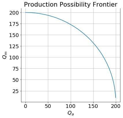
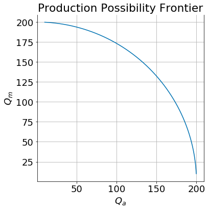
Notice that we can invert the two production function to get minimum labor requirement functions \(L_a(Q_a)\) and \(L_m(Q_m)\) which tell us the minimum amount of labor \(L_i\) required in sector \(i\) to produce quantity \(Q_i\). If we take these expressions and substitute them into the labor resource constraint we get an expression for the production possibility frontier (PPF) which summarizes the tradeoffs between sectors.

Assumptions and parameters for visualizations

Let’s get concrete and assume each sector employs a CRS Cobb-Douglas production function:

\[F(\bar T, L_a)=\bar T^{1-\alpha} \cdot L_a^\alpha\]

\[G(\bar K, L_m)=\bar K^{1-\beta} \cdot L_m^\beta\]

If \(\alpha = \beta = \frac{1}{2}\) and \(\bar T= \bar K = 100\). Then

\[Q_a = \sqrt{\bar T} \sqrt{L_a}\]

\[Q_m = \sqrt{\bar K} \sqrt{L_m}\]

Substituting these into the labor resource constraint yields:

\[\frac{Q_a^2}{\bar T}+\frac{Q_m^2}{\bar K} = \bar L\]

or

\[Q_m = \sqrt{\bar K \bar L - \frac{\bar K Q_a^2}{\bar T} }\]

If we make the further assumption that \(\bar K = \bar L = 100\) and \(\bar L = 400\) then the PPF would look like this:

NOTE: If you are running this as a live jupyter notebook please first go to the code section below and execute all the code cells there. Then return and run the code cells that follow sequentially.

ppf(Tbar=100, Kbar=100, Lbar=400)

Labor market equilibrium

Profit maximizing firms in each sector will hire labor up to the point where the marginal value product of labor (MVPL) equals the market wage. Since labor is mobile across sectors in equilibrium workers must be paid the same nominal wage \(w\) in either sector:

\[P_a \cdot MPL_a(\bar T, L_a) = w = P_m \cdot MPL_m(\bar K, L_m)\]

It will be useful to express the wage in real terms. Divide each expression above by \(P_m\) to get

\[p \cdot MPL_a = \frac{w}{p_m} = MPL_m\]

\[\text{ where } p = \frac{P_a}{P_m}\]

In the plots below we will place the real wage measured in terms of manufactured goods on the vertical axis of the labor demand and supply diagrams.

Labor allocation across sectors

In a competitive market firms take the market prices of goods \(p\) and wages \(w\) as given. Since in equilibrium the labor market clears we can write \(L_m = \bar L - L_a\) and substitute into the equilibrium condition above to get:

\[p \cdot MPL_a(L_A) = w = MPL_m(\bar L-L_A)\]

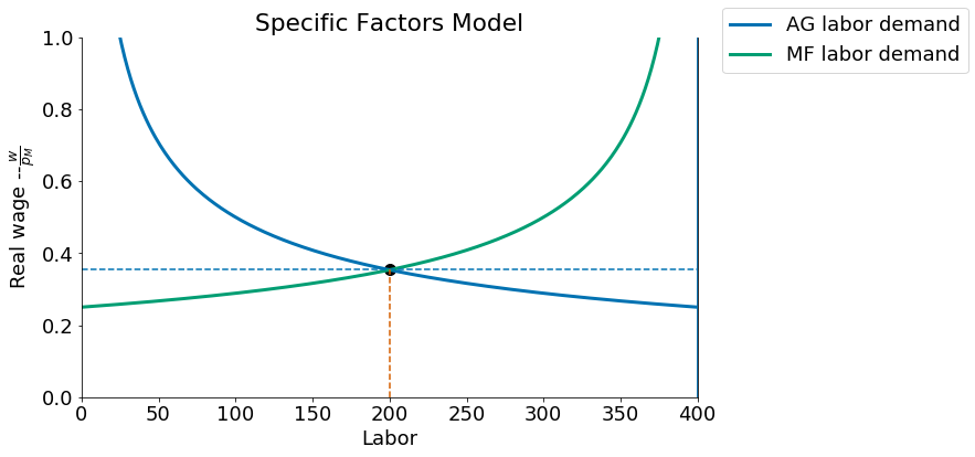
The left hand side \(p \cdot MPL_a(L_A)=w\) can be solved to give us demand for labor in the agricultural sector as a function of the wage \(L_a(w/p)\) and is plotted below. The right hand side \(w = MPL_m(\bar L-L_a)\) gives us demand for labor in the manufacturing sector \(L_m\) as a function of the real wage but this in turn also gives us the supply of labor to the agricultural sector \(L_a^s = \bar L - L_m(w/p)\) since firms in the agricultural sector can only attract workers to their sector by paying those workers just a bit above what they would be paid for the jobs they have to leave in the manufacturing sector.

The diagram below can therefore be interpreted as showing labor demand and supply in the agricultural sector and their intersection gives us the equilibrium real wage (measured on the vertical in terms of purchasing power over manufactured goods).

sfmplot(p=1)

(La, Lm) = (200, 200)   (w/Pm, w/Pa) =(0.35, 0.35)
(v/Pa, v/Pm) = (0.7, 0.7)   (r/Pa, r/Pm) = (0.7, 0.7)

We can solve for the equilibrium labor allocation \(L_a\) as a function of the relative price \(p\), and this in turn also gives us the equilibrium real wage. When \(\alpha=\beta = \frac{1}{2}\) the equilibrium condition \(p \cdot MPL_a(L_a) = MPL_m(\bar L-L_a)\) becomes:

\[p \cdot \frac{\sqrt{\bar T}}{\sqrt{L_a}} = \frac{\sqrt{\bar K}}{\sqrt{\bar L - L_a}}\]

which we solve to find:

\[L_a^e = \frac{p^2 \bar T \bar L}{\bar K - p^2 \bar T}\]

For cases where \(\alpha \ne \beta\) we find the optimal \(L_a\) that solves this equilibrium condition numerically.

Autarky prices

Thus far we have a pretty complete model of how production allocations and real wages would be determined in a small open economy where producers face world price ratio \(p\). we explore comparative statics in this economy in more detail below.

If however the economy is inititally in autarky or closed to the world then we must also consider the role of domestic consumer preferences in the determination of domestic equilibrium product prices.

With Cobb-Douglas preferences \(u(x,y) = \gamma \ln(x) + (1-\gamma) \ln(y)\) consumers demands can be written as a function of relative price \(p=\frac{P_a}{P_m}\). Setting \(P_m=1\) to make manufacturing the numeraire good, this can be written:

\[\begin{split}\begin{align} C_a(p) =& \gamma \cdot \frac{I(p)}{p} \\ C_m(p) =& (1-\gamma) \cdot I(p) \end{align}\end{split}\]

Income \(I\) in the expressions is given by the value of national production or GDP at these prices. Measured in manufactured goods:

\[I(p) = p \cdot F(\bar T, L_a(p)) + G(\bar K, \bar L - L_a(p)\]

By Walras’ law we only need to find the relative price at which output equals demand in one of the two product markets so in the the code below we solve for equilibrium domestic prices from the condition \(Q_a(p)=C_a(p)\).

For parameters \(\alpha=\beta=\gamma = \frac{1}{2}\), \(\bar T = \bar K =100\) and \(\bar L=400\) the domestic equilibrium prices are unitary:

p_autarky(Lbar, Tbar, Kbar)

1.0

And this in turn leads to an equilibrium autarky allocation with \(L_a = L_m = 200\) and a real wage \(\frac{w}{p}=0.35\).

eqn(p_autarky())

(200.0, 0.35355339059327373)

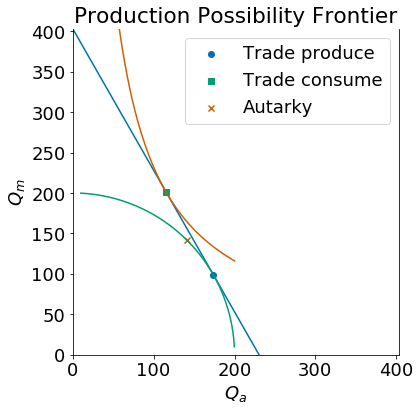
The plot below shows the autarky production and consumption point (marked by an ‘X’) as well as the new production point (marked by a circle) and consumption point (marked by a square) if the country opened to trade with a world relative price \(p=\frac{7}{4}\).

Opening to trade leads the country to expand agricultural production by re-allocating labor from manufacturing to agriculture. We confirm the expected neoclassical ambiguity result which is that an increase in the relative price of agricultural goods will lead to an increase in the real wage measured in terms of manufactured goods \(\frac{w}{p_m}\) (\(=w\) since we have \(P_m=1\)) but a decrease in real wage measured in terms of agricultural goods or \(\frac{w}{P_a} = \frac{w}{p}\) in our notation (since \(\frac{w}{P_a} = \frac{w}{p_m} \cdot \frac{P_m}{P_a}\)).

Diagrammatically

\[p \uparrow \rightarrow \frac{w}{p_m} \uparrow , \frac{w}{p_a} \downarrow\]

pw = 7/4
Lao, wo = eqn(p=pw)
Lao, wo, wo/pw

(301.53846153846149, 0.50389110926865943, 0.28793777672494825)

sfmtrade(p=7/4)

Effects of a price change on the income distribution

More explanations to be placed here…

sfmplot2(2)

## Code Section

Make sure you run the cells below FIRST. Then run the cells above

Python simulation and plots

import numpy as np
from scipy.optimize import fsolve
np.seterr(divide='ignore', invalid='ignore')
import matplotlib.pyplot as plt
from ipywidgets import interact, fixed
import seaborn
%matplotlib inline

plt.style.use('seaborn-colorblind')
plt.rcParams["figure.figsize"] = [7,7]
plt.rcParams["axes.spines.right"] = True
plt.rcParams["axes.spines.top"] = False
plt.rcParams["font.size"] = 18
plt.rcParams['figure.figsize'] = (10, 6)
plt.rcParams['axes.grid']=True

Tbar = 100       # Fixed specific land in ag.
Kbar = 100       # Fixed specific capital in manuf
Lbar = 400       # Total number of mobile workers
LbarMax = 400    # Lbar will be on slider, max value.

p    = 1.00      # initial rel price of ag goods, p = Pa/Pm
alpha, beta = 0.5, 0.5  # labor share in ag, manuf

For the plots we want to plot over \(L_a\) and \(L_m = \bar L -l_a\):

La = np.linspace(1, LbarMax-1,LbarMax)
Lm = Lbar - La

The production functions in each sector:

def F(La, Tbar = Tbar):
    return (Tbar**(1-alpha) * La**alpha)

def G(Lm, Kbar =Kbar):
    return (Kbar**(1-beta) * Lm**beta)

def MPLa(La):
    return alpha*Tbar**(1-alpha) * La**(alpha-1)

def MPLm(Lm):
    return beta*Kbar**(1-beta) * Lm**(beta-1)

def MPT(La, Tbar=Tbar):
    return (1-alpha)*Tbar**(-alpha) * La**alpha

def MPK(Lm, Kbar=Kbar):
    return (1-beta)*Kbar**(-beta) * Lm**beta

We have enough to plot a production possibility Frontier (and how it varies with factor supplies):

def ppf(Tbar=Tbar, Kbar=Kbar, Lbar=Lbar):
    Qa = F(La, Tbar) * (La<Lbar)
    Qm = G(Lm, Kbar)
    plt.title('Production Possibility Frontier')
    plt.xlabel(r'$Q_a$')
    plt.ylabel(r'$Q_m$')
    plt.plot(Qa, Qm)
    plt.gca().set_aspect('equal');

ppf(Tbar=100, Kbar=100, Lbar=400)

Labor demand in each sector as a function of \(p=\frac{P_a}{P_m}\):

LDa = p * MPLa(La) *(La<Lbar)         # for Cobb-Douglas MPL can be written this way
LDm = MPLm(Lbar-La)

The following function returns the equilibrium allocation of labor to agriculture and equilibrium nominal wage for any initial relative price of agricultural goods \(p=\frac{P_a}{P_m}\)

def eqn(p, Lbar=Lbar):
    '''returns numerically found equilibrium labor allocation and wage'''
    def func(La):
        return p*MPLa(La) - MPLm(Lbar-La)
    Laeq = fsolve(func, 1)[0]
    return Laeq, p*MPLa(Laeq)

def u(x,y):
    '''Utility function'''
    return x*y

def XD(p, Lbar = Lbar):
    '''Cobb-Douglas demand for goods given world prices (national income computed)'''
    LAe, we = eqn(p)
    # gdp at world prices measured in manuf goods
    gdp = p*F(LAe, Tbar = Tbar) + G(Lbar -LAe, Kbar=Kbar)
    return (1/2)*gdp/p, (1/2)*gdp

def indif(x, ubar):
    return ubar/x

def p_autarky(Lbar=Lbar, Tbar=Tbar, Kbar=Kbar):
    '''Find autarky product prices. By Walras' law enough to find price that
    sets excess demand in just one market'''
    def excessdemandA(p):
        LAe, _ = eqn(p)
        QA = F(LAe, Tbar = Tbar)
        CA, CM = XD(p, Lbar=Lbar)
        return QA-CA
    peq = fsolve(excessdemandA, 1)[0]
    return peq

p_autarky()

1.0

def sfmtrade(p):
    Ca = np.linspace(0,200,200)
    LAe, we = eqn(p)
    X, Y = F(LAe, Tbar = Tbar), G(Lbar -LAe)
    gdp = p*X + Y
    plt.scatter(F(LAe, Tbar), G(Lbar-LAe, Tbar), label='Trade produce')
    plt.scatter(*XD(p),label='Trade consume', marker='s')
    plt.scatter(*XD(p_autarky()), marker='x', label='Autarky')
    plt.plot([0,gdp/p],[gdp, 0])
    ppf(100)
    ub = u(*XD(p))
    plt.ylim(0,gdp)
    plt.xlim(0,gdp)
    plt.plot(Ca, indif(Ca, ub))
    plt.grid(False)
    plt.legend()
    plt.gca().spines['bottom'].set_position('zero')
    plt.gca().spines['left'].set_position('zero')

sfmtrade(p=7/4)

Simple example with \(\bar L\) at \(\bar L^{max}\)

La = np.arange(0, LbarMax)   # this is always over the LbarMax range

def sfmplot(p, Lbar=LbarMax, show=True):
    Lm = Lbar - La
    Qa = (Tbar**(1-alpha) * La**alpha) * (La<Lbar)
    Qm = Kbar**(1-beta) * (Lbar - La)**beta
    pMPLa = (p * alpha * Qa/La)*(La<Lbar)         # for Cobb-Douglass MPL can be written this way
    MPLm = beta * Qm/(Lbar-La)
    LA, weq = eqn(p)
    ymax = 1.0
    plt.ylim(0,ymax)
    plt.xlim(0,LbarMax)
    plt.title('Specific Factors Model')
    plt.plot(La, pMPLa, linewidth = 3, label='AG labor demand')
    plt.plot(La, MPLm, linewidth=3, label ='MF labor demand')
    plt.scatter(LA, weq, s=100, color='black')
    plt.axhline(weq, linestyle='dashed')
    plt.axvline(Lbar, linewidth = 3)
    plt.plot([LA, LA],[0, weq], linestyle='dashed')
    plt.xlabel('Labor')
    plt.ylabel('Real wage --' + r'$\frac{w}{p_M}$')
    plt.grid()
    if show:
        plt.legend(loc=(1.04,0.9))
        print("(La, Lm) = ({0:3.0f}, {1:3.0f})   (w/Pm, w/Pa) =({2:3.2f}, {3:3.2f})"
              .format(LA, Lbar-LA, weq, weq/p))
        print("(v/Pa, v/Pm) = ({0:3.1f}, {1:3.1f})   (r/Pa, r/Pm) = ({2:3.1f}, {3:3.1f})"
              .format(MPT(LA), p*MPT(LA), MPK(Lbar-LA)/p, MPK(Lbar-LA)    )   )
        plt.show()

If you are wondering about why we skip the plt.show() when show=True, it’s because for figures that use the ipywidgets interact function to allow parameters to change with sliders we will need to have a plt.show() to redraw the plot in every function call (otherwise we would end up with a stack of plots rather than a changing plot).

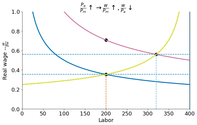
sfmplot(p=2)

(La, Lm) = (320,  80)   (w/Pm, w/Pa) =(0.56, 0.28)
(v/Pa, v/Pm) = (0.9, 1.8)   (r/Pa, r/Pm) = (0.2, 0.4)

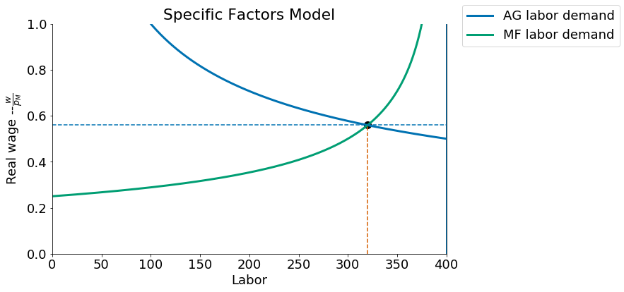
Suppose that by opening to trade the relative price of agricultural goods \(p\) doubles from \(p=1\) to \(p=2\). This greatly shifts the demand for agricultural workers:

def sfmplot2(p):
    sfmplot(1, show=False)
    sfmplot(p, show=False)
    plt.grid(False)
    if p == 1:
        plt.title('SF Model');
    else:
        La0, w0 = eqn(1)
        plt.scatter(La0,w0*p, s=100, color='black')  #where wage would rise to without labor movement
        if p>1:
            plt.title(r'$\frac{P_a}{P_m} \uparrow  \rightarrow  \frac{w}{P_m} \uparrow, \frac{w}{P_a} \downarrow $'  );
        elif p<1:
            plt.title(r'$\frac{P_a}{P_m} \downarrow  \rightarrow  \frac{w}{P_m} \downarrow, \frac{w}{P_a} \uparrow $'  );
    plt.show();

sfmplot2(2)

interact(sfmplot2, p=(0.1, 2,0.1));

Before and after plots

The trick here is to define a new plotting function that first plots a static plot and then allows an interaction.

interact(sfmplot2, p=(0,2,0.2), Lbar=fixed(400), show=fixed(True))

<function __main__.sfmplot2>