Stata and R in a jupyter notebook
The jupyter notebook project is now designed to be a ‘language agnostic’ web-application front-end for any one of many possible software language kernels. We’ve been mostly using python but there are in fact several dozen other language kernels that can be made to work with it including Julia, R, Matlab, C, Go, Fortran and Stata.
The ecosystem of libraries and packages for scientific computing with python is huge and constantly growing but there are still many statistics and econometrics applications that are available as built-in or user-written modules in Stata that have not yet been ported to python or are just simply easier to use in Stata. On the other hand there are some libraries such as python pandas and different visualization libraries such as seaborn or matplotlib that give features that are not available in Stata.
Fortunately you don’t have to choose between using Stata or python, you can use them both together, to get the best of both worlds.
Jupyter running an R kernel
R is a powerful open source software environment for statistical computing. R has R markdown which allows you to create R-markdown notebooks similar in concept to jupyter notebooks. But you can also run R inside a jupyter notebook (indeed the name ‘Jupyter’ is from Julia, iPython and R).
See my notebook with notes on Research Discontinuity Design for an example of a jupyter notebook running R. To install an R kernel see the IRkernel project.
Jupyter with a Stata Kernel
Kyle Barron has created a stata_kernel that offers several useful features including code-autocompletion, inline graphics, and generally fast responses.
For this to work you must have a working licensed copy of Stata version 14 or greater on your machine.
Python and Stata combined in the same notebook
Sometimes it may be useful to combine python and Stata in the same
notebook. Ties de Kok has written a nice python library called
ipystata that allows one to
execute Stata code in codeblocks inside an ipython notebook when
preceded by a %%stata magic command.
This workflow allows you to pass data between python and Stata sessions and to display Stata plots inline. Compared to the stata_kernel option the response times are not quite as fast.
The remainder of this notebook illustrates the use of ipystata.
A sample ipystata session
For more details see the example notebook and documentation on the ipystata repository.
In [1]:
%matplotlib inline
import seaborn as sns
import pandas as pd
import statsmodels.formula.api as smf
import ipystata
The following opens a Stata session where we load a dataset and
summarize the data. The -o flag following the `%%Stata``` magic
instructs it to output or return the dataset in Stata memory as a pandas
dataframe in python.
In [2]:
%%stata -o life_df
sysuse lifeexp.dta
summarize
(Life expectancy, 1998)

    Variable |        Obs        Mean    Std. Dev.       Min        Max
-------------+---------------------------------------------------------
      region |         68         1.5    .7431277          1          3
     country |          0
   popgrowth |         68    .9720588    .9311918        -.5          3
        lexp |         68    72.27941    4.715315         54         79
       gnppc |         63    8674.857    10634.68        370      39980
-------------+---------------------------------------------------------
   safewater |         40        76.1    17.89112         28        100
Let’s confirm the data was returned as a pandas dataframe:
In [3]:
life_df.head(3)
Out[3]:
| region | country | popgrowth | lexp | gnppc | safewater | |
|---|---|---|---|---|---|---|
| 0 | Eur & C.Asia | Albania | 1.2 | 72 | 810.0 | 76.0 |
| 1 | Eur & C.Asia | Armenia | 1.1 | 74 | 460.0 | NaN |
| 2 | Eur & C.Asia | Austria | 0.4 | 79 | 26830.0 | NaN |
A simple generate variable command and ols regression in Stata:
In [4]:
%%stata -o life_df
gen lngnppc = ln(gnppc)
regress lexp lngnppc
(5 missing values generated)

      Source |       SS           df       MS      Number of obs   =        63
-------------+----------------------------------   F(1, 61)        =     97.09
       Model |  873.264865         1  873.264865   Prob > F        =    0.0000
    Residual |  548.671643        61  8.99461709   R-squared       =    0.6141
-------------+----------------------------------   Adj R-squared   =    0.6078
       Total |  1421.93651        62  22.9344598   Root MSE        =    2.9991

------------------------------------------------------------------------------
        lexp |      Coef.   Std. Err.      t    P>|t|     [95% Conf. Interval]
-------------+----------------------------------------------------------------
     lngnppc |   2.768349   .2809566     9.85   0.000     2.206542    3.330157
       _cons |   49.41502   2.348494    21.04   0.000     44.71892    54.11113
------------------------------------------------------------------------------
And the same regression using statsmodels and pandas:
In [5]:
model = smf.ols(formula = 'lexp ~ lngnppc',
                data = life_df)
results = model.fit()
print(results.summary())
                            OLS Regression Results
==============================================================================
Dep. Variable:                   lexp   R-squared:                       0.614
Model:                            OLS   Adj. R-squared:                  0.608
Method:                 Least Squares   F-statistic:                     97.09
Date:                Tue, 08 May 2018   Prob (F-statistic):           3.13e-14
Time:                        14:25:48   Log-Likelihood:                -157.57
No. Observations:                  63   AIC:                             319.1
Df Residuals:                      61   BIC:                             323.4
Df Model:                           1
Covariance Type:            nonrobust
==============================================================================
                 coef    std err          t      P>|t|      [0.025      0.975]
------------------------------------------------------------------------------
Intercept     49.4150      2.348     21.041      0.000      44.719      54.111
lngnppc        2.7683      0.281      9.853      0.000       2.207       3.330
==============================================================================
Omnibus:                       21.505   Durbin-Watson:                   1.518
Prob(Omnibus):                  0.000   Jarque-Bera (JB):               46.140
Skew:                          -1.038   Prob(JB):                     9.57e-11
Kurtosis:                       6.643   Cond. No.                         52.7
==============================================================================

Warnings:
[1] Standard Errors assume that the covariance matrix of the errors is correctly specified.
Back to ipython
Let’s change one of the variables in the dataframe in python:
In [6]:
life_df.popgrowth = life_df.popgrowth * 100
In [7]:
life_df.popgrowth.mean()
Out[7]:
97.20587921142578
And now let’s push the modified dataframe into the Stata dataset with
the -d flag:
In [8]:
%%stata -d life_df
summarize
    Variable |        Obs        Mean    Std. Dev.       Min        Max
-------------+---------------------------------------------------------
       index |         68        33.5    19.77372          0         67
      region |         68          .5    .7431277          0          2
     country |          0
   popgrowth |         68    97.20588    93.11918        -50        300
        lexp |         68    72.27941    4.715315         54         79
-------------+---------------------------------------------------------
       gnppc |         63    8674.857    10634.68        370      39980
   safewater |         40        76.1    17.89112         28        100
     lngnppc |         63    8.250023    1.355677   5.913503   10.59613
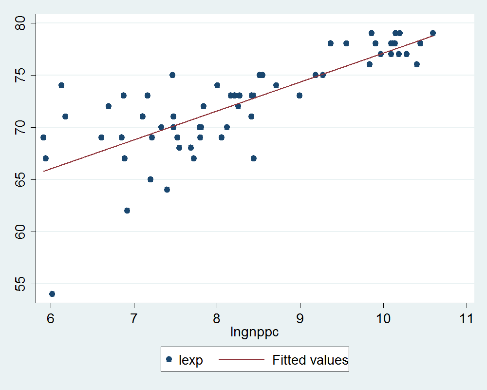
A Stata plot:
In [9]:
%%stata -d life_df --graph
graph twoway (scatter lexp lngnppc) (lfit lexp lngnppc)
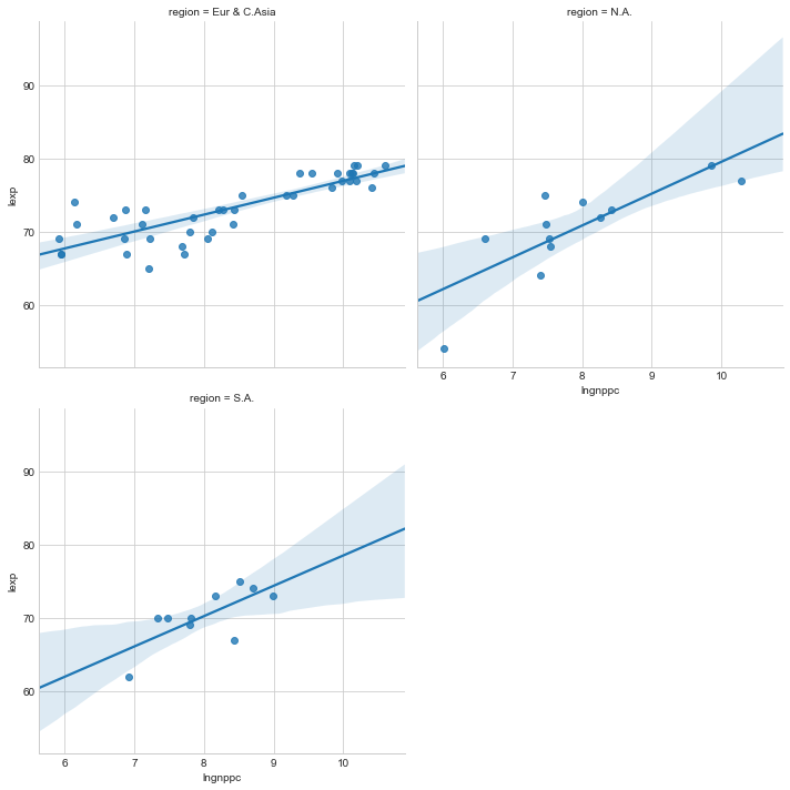
Now on the python side use lmplot from the seaborn library to graph a similar scatter and fitted line but by region.
In [10]:
sns.set_style("whitegrid")
g=sns.lmplot(y='lexp', x='lngnppc', col='region', data=life_df,col_wrap=2)